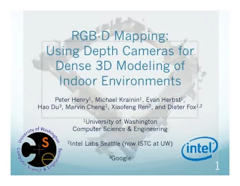
Mapping and Modeling with RGB-D Cameras University of Washington - PowerPoint PPT Presentation
Mapping and Modeling with RGB-D Cameras University of Washington Dieter Fox 1 Outline Motivation RGB-D Mapping: 1. Visual Odometry (frame-to-frame alignment) 2. Loop Closure (revisiting places) 3. Map representation (Surfels) 2
Mapping and Modeling with RGB-D Cameras University of Washington Dieter Fox 1
Outline • Motivation • RGB-D Mapping: 1. Visual Odometry (frame-to-frame alignment) 2. Loop Closure (revisiting places) 3. Map representation (Surfels) 2
Outline • Motivation • RGB-D Mapping: 1. Visual Odometry (frame-to-frame alignment) 2. Loop Closure (revisiting places) 3. Map representation (Surfels) 3
RGB-D (Kinect-style) Cameras 4
Multisense SL 5
Velodyne & LadyBug3 6
Motivation • Tracking RGB-D camera motion and creating a 3D model has applications for – Rich interior maps – Robotics • Localization / Mapping • Manipulation – Augmented reality – 3D content creation 7
Goal • Track the 3D motion of an RGB-D camera • Build a useful and accurate model of the environment 8
Outline • Motivation • RGB-D Mapping: 1. Frame-to-frame motion (visual odometry) 2. Revisiting places (loop closure detection) 3. Map representation (Surfels) 9
RGB-D Mapping Overview Map `` RGB-D Mapping: Using Depth Cameras for Dense 3D Modeling of Indoor Environments. Henry et al. ISER 2010 RGB-D Mapping: Using Kinect-style Depth Cameras for Dense 3D Modeling of Indoor Environments. Henry et al. IJRR 2012 10
Visual Odometry • Compute the motion between consecutive camera frames from visual feature correspondences. • Visual features from RGB image have a 3D counterpart from depth image. 11
Visual Features • Tree bark itself not really distinct • Rocky ground not distinct • Rooftops, windows, lamp post fairly distinct and should be easier to match across images Say we have 2 images of this scene we’d like to align by matching local features What would be good local features (ones easy to match)? Courtesy: S. Seitz and R. Szeliski
Invariant local features -Algorithm for finding points and representing their patches should produce similar results even when conditions vary - Buzzword is “invariance” – geometric invariance: translation, rotation, scale – photometric invariance: brightness, exposure, … Feature Descriptors Courtesy: S. Seitz and R. Szeliski
Robust visual features • Goal: Detect distinctive features, maximizing repeatability – Scale invariance • Robust to changes in distance – Rotation invariance • Robust to rotations of camera – Affine invariance • Robust to tilting of camera – Brightness invariance • Robust to minor changes in illumination – Produce small descriptors that can be compared using simple mathematical operations • (SSE) • Euclidean distance 14
Scale Invariant Detection • Consider regions (e.g. circles) of different sizes around a point • Regions of corresponding sizes will look the same in both images
Scale Invariant Detection • The problem: how do we choose corresponding circles independently in each image?
Scale Invariant Detection • Solution: – Design a function on the region (circle), which is “scale invariant” (the same for corresponding regions, even if they are at different scales) Example: average intensity. For corresponding regions (even of different sizes) it will be the same.
Scale Invariant Detection • Solution: – Design a function on the region (circle), which is “scale invariant” (the same for corresponding regions, even if they are at different scales) Example: average intensity. For corresponding regions (even of different sizes) it will be the same. – For a point in one image, we can consider it as a function of region size (circle radius) Image 1 f f Image 2 scale = 1/2 region size region size
Scale Invariant Detection • Common approach: Take a local maximum of this function Observation : region size, for which the maximum is achieved, should be invariant to image scale. Important: this scale invariant region size is found in each image independently! Image 1 f f Image 2 scale = 1/2 s 1 s 2 region size region size
Scale Invariant Detection • A “good” function for scale detection: has one stable sharp peak f f f Good ! bad bad region size region size region size • For usual images: a good function would be a one which responds to contrast (sharp local intensity change)
Scale Invariant Detection f • Functions for determining scale Kernel Image Kernels: 2 L G ( , , ) x y G ( , , ) x y xx yy (Laplacian of Gaussians) DoG G x y k ( , , ) G x y ( , , ) (Difference of Gaussians) where Gaussian 2 2 x y Note: both kernels are invariant 2 1 2 G x y ( , , ) e to scale and rotation 2
Scale Invariant Detectors scale • Harris-Laplacian 1 Laplacian Find local maximum of: – Harris corner detector in y space (image coordinates) – Laplacian in scale Harris x scale • SIFT (Lowe) 2 DoG Find local maximum of: – Difference of Gaussians in space and scale y DoG x 1 K.Mikolajczyk, C.Schmid . “Indexing Based on Scale Invariant Interest Points”. ICCV 2001 2 D.Lowe . “Distinctive Image Features from Scale -Invariant Keypoints ”. IJCV 2004
Lindeberg et al, 1996 Lindeberg et al., 1996 Slide from Tinne Tuytelaars Slide from Tinne Tuytelaars
Slide from Tinne Tuytelaars
Slide from Tinne Tuytelaars
Slide from Tinne Tuytelaars
Slide from Tinne Tuytelaars
Slide from Tinne Tuytelaars
Slide from Tinne Tuytelaars
Slide from Tinne Tuytelaars
Feature descriptors We now know how to detect good points Next question: How to match them? ? Courtesy: S. Seitz and R. Szeliski
Feature descriptors We now know how to detect good points Next question: How to match them? ? Point descriptor should be: 1. Invariant 2. Distinctive Courtesy: S. Seitz and R. Szeliski
Invariance • Suppose we are comparing two images I 1 and I 2 – I 2 may be a transformed version of I 1 – What kinds of transformations are we likely to encounter in practice?
Invariance • Suppose we are comparing two images I 1 and I 2 – I 2 may be a transformed version of I 1 – What kinds of transformations are we likely to encounter in practice? • Translation, 2D rotation, scale
Invariance • Suppose we are comparing two images I 1 and I 2 – I 2 may be a transformed version of I 1 – What kinds of transformations are we likely to encounter in practice? • Translation, 2D rotation, scale • Descritpors can usually also handle – Limited 3D rotations ( SIFT works up to about 60 degrees) – Limited affine transformations (2D rotation, scale, shear) – Limited illumination/contrast changes
How to achieve invariance Need both of the following: 1. Make sure your detector is invariant – SIFT is invariant to translation, rotation and scale 2. Design an invariant feature descriptor – A descriptor captures the information in a region around the detected feature point
Scale Invariant Feature Transform • Algorithm outline: – Detect interest points – For each interest point • Determine dominant orientation • Build histograms of gradient directions • Output feature descriptor 37
Scale Invariant Feature Transform Basic idea: • Take 16x16 square window around detected feature • Compute gradient for each pixel • Throw out weak gradient magnitudes • Create histogram of surviving gradient orientations 2 0 angle histogram Adapted from slide by David Lowe
SIFT keypoint descriptor Full version • Divide the 16x16 window into a 4x4 grid of cells (2x2 case shown below) • Compute an orientation histogram for each cell • 16 cells * 8 orientations = 128 dimensional descriptor Adapted from slide by David Lowe
Properties of SIFT Extraordinarily robust matching technique – Can handle changes in viewpoint • Up to about 60 degree out of plane rotation – Can handle significant changes in illumination • Sometimes even day vs. night (below) – Fast and efficient — can run in real time – Lots of code available • http://www.vlfeat.org • http://www.cs.unc.edu/~ccwu/siftgpu/
Feature matching Given a feature in I 1 , how to find the best match in I 2 ? 1. Define distance function that compares two descriptors 2. Test all the features in I 2 , find the one with min distance
Feature distance • How to define the difference between two features f1, f2? – Simple approach is SSD(f1, f2) • sum of square differences between entries of the two descriptors • can give good scores to very ambiguous (bad) matches f 1 f 2 I 1 I 2
Feature distance • How to define the difference between two features f1, f2? – Better approach: ratio distance = SSD(f1, f2) / SSD(f1, f2’) • f2 is best SSD match to f1 in I 2 • f2’ is 2nd best SSD match to f1 in I 2 • gives small values for ambiguous matches ' f 1 f 2 f 2 I 1 I 2
Lots of applications Features are used for: – Image alignment (e.g., mosaics) – 3D reconstruction – Motion tracking – Object recognition – Indexing and database retrieval – Robot navigation – … other
More Features • FAST • GFTT • SURF • ORB • STAR • MSER • KAZE http://computer-vision-talks.com/articles/2011-07-13-comparison-of-the-opencv-feature-detection-algorithms/ • A-KAZE 45
Are descriptors unique? 46
Recommend
More recommend
Explore More Topics
Stay informed with curated content and fresh updates.
