R01 - Simple linear regression STAT 587 (Engineering) Iowa State - PowerPoint PPT Presentation

R01 - Simple linear regression STAT 587 (Engineering) Iowa State University October 17, 2020

Simple linear regression Telomere length Telomere length http://www.pnas.org/content/101/49/17312 People who are stressed over long periods tend to look haggard, and it is commonly thought that psycholog- ical stress leads to premature aging [as measured by decreased telomere length] ... examine the importance of ... caregiving stress (...num- ber of years since a child’s diagnosis [of a chronic dis- ease]) [on telomere length] ... Telomere length values were measured from DNA by a quantitative PCR assay that determines the relative ra- tio of telomere repeat copy number to single-copy gene copy number (T/S ratio) in experimental samples as compared with a reference DNA sample.

Simple linear regression Telomere length Data Telomere length vs years post diagnosis 1.6 1.4 Telomere length 1.2 1.0 2.5 5.0 7.5 10.0 12.5 Years since diagnosis (jittered)

Simple linear regression Telomere length Data with regression line Telomere length vs years post diagnosis 1.6 1.4 Telomere length 1.2 1.0 2.5 5.0 7.5 10.0 12.5 Years since diagnosis (jittered)

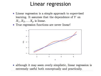
Simple linear regression Model Simple Linear Regression The simple linear regression model is ind ∼ N ( β 0 + β 1 X i , σ 2 ) Y i where Y i and X i are the response and explanatory variable, respectively, for individual i . Terminology (all of these are equivalent): response explanatory outcome covariate dependent independent endogenous exogenous

Simple linear regression Model Simple linear regression - visualized Simple linear regression model Response variable Explanatory variable

Simple linear regression Parameter interpretation Parameter interpretation Recall: V ar [ Y i | X i = x ] = σ 2 E [ Y i | X i = x ] = β 0 + β 1 x If X i = 0 , then E [ Y i | X i = 0] = β 0 . β 0 is the expected response when the explanatory variable is zero. If X i increases from x to x + 1 , then E [ Y i | X i = x + 1] = β 0 + β 1 x + β 1 − E [ Y i | X i = x ] = β 0 + β 1 x = β 1 β 1 is the expected increase in the response for each unit increase in the explanatory variable. σ is the standard deviation of the response for a fixed value of the explanatory variable.

Simple linear regression Parameter interpretation Simple linear regression - visualized Simple linear regression model 12 8 Response variable 4 0 0 2 4 6 8 Explanatory variable

Simple linear regression Parameter estimation Remove the mean: iid ∼ N (0 , σ 2 ) Y i = β 0 + β 1 X i + e i e i So the error is e i = Y i − ( β 0 + β 1 X i ) which we approximate by the residual e i = Y i − (ˆ β 0 + ˆ r i = ˆ β 1 X i ) The least squares (minimize � n i =1 r 2 i ), maximum likelihood, and Bayesian estimators (prior 1 /σ 2 ) are ˆ β 1 = SXY/SXX ˆ = Y − ˆ β 0 β 1 X σ 2 ˆ = SSE/ ( n − 2) d f = n − 2 � n = 1 X i =1 X i n � n = 1 Y i =1 Y i n = � n SXY i =1 ( X i − X )( Y i − Y ) = � n i =1 ( X i − X )( X i − X ) = � n i =1 ( X i − X ) 2 SXX = � n i =1 r 2 SSE i

Simple linear regression Parameter estimation Residuals Telomere length vs years post diagnosis 1.6 1.4 Telomere length 1.2 1.0 2.5 5.0 7.5 10.0 12.5 Years since diagnosis (jittered)

Simple linear regression Parameter estimation Residuals Telomere length vs years post diagnosis 1.6 1.4 Telomere length 1.2 1.0 2.5 5.0 7.5 10.0 12.5 Years since diagnosis (jittered)

Simple linear regression Standard errors How certain are we about ˆ β 0 and ˆ β 1 ? We quantify this uncertainty using their standard errors (or posterior scale parameters): � 2 SE (ˆ 1 X β 0 ) = ˆ σ n + d f = n − 2 ( n − 1) s 2 X SE (ˆ � 1 β 1 ) = ˆ σ d f = n − 2 ( n − 1) s 2 X s 2 = SXX/ ( n − 1) X s 2 = SY Y/ ( n − 1) Y = � n i =1 ( Y i − Y ) 2 SY Y = SXY/ ( n − 1) r XY correlation coefficient s X s Y R 2 = r 2 XY = SST − SSE coefficient of determination SST = SY Y = � n i =1 ( Y i − Y ) 2 SST The coefficient of determination ( R 2 ) is the proportion of the total response variation explained by the model.

Simple linear regression Standard errors Default Bayesian analysis of the simple linear regression model If we assume the default prior p ( β 0 , β 1 , σ 2 ) ∝ 1 /σ 2 , then the marginal posteriors for the mean parameters are β j | y ∼ t n − 2 (ˆ β j , SE (ˆ β j ) 2 ) . We can construct a 100(1 − a )% two-sided credible interval for β j via β j ± t n − 2 , 1 − a/ 2 SE (ˆ ˆ β j ) where P ( T n − 2 < t n − 2 , 1 − a/ 2 ) = 1 − a/ 2 for T n − 2 ∼ t n − 2 . We can compute posterior probabilities via ˆ � � β j − b j P ( β j < b j | y ) = P T n − 2 < SE ( ˆ β j ) ˆ � � β j − b j P ( β j > b j | y ) = P T n − 2 > . SE ( ˆ β j )

Simple linear regression p -values and confidence intervals p -values and confidence interval We can construct a 100(1 − a )% two-sided confidence interval for β j via β j ± t n − 2 , 1 − a/ 2 SE (ˆ ˆ β j ) . We can compute one-sided p -values, e.g. H 0 : β j ≥ b j vs H A : β j < b j has � � ˆ β j − b j p -value = P T n − 2 > SE (ˆ β j ) and H 0 : β j ≤ b j vs H A : β j > b j has � � ˆ β 1 − b j p -value = P T n − 2 < SE (ˆ β j ) software default is usually b j = 0 .

Simple linear regression by hand Calculations “by hand” in R n = nrow(Telomeres) Xbar = mean(Telomeres$years) Ybar = mean(Telomeres$telomere.length) s_X = sd(Telomeres$years) s_Y = sd(Telomeres$telomere.length) r_XY = cor(Telomeres$telomere.length, Telomeres$years) SXX = (n-1)*s_X^2 SYY = (n-1)*s_Y^2 SXY = (n-1)*s_X*s_Y*r_XY beta1 = SXY/SXX beta0 = Ybar - beta1 * Xbar R2 = r_XY^2 SSE = SYY*(1-R2) sigma2 = SSE/(n-2) sigma = sqrt(sigma2) SE_beta0 = sigma*sqrt(1/n + Xbar^2/((n-1)*s_X^2)) SE_beta1 = sigma*sqrt( 1/((n-1)*s_X^2))

Simple linear regression by hand Calculations “by hand” in R (continued) # 95% CI for beta0 beta0 + c(-1,1)*qt(.975, df = n-2) * SE_beta0 [1] 1.251761 1.483603 # 95% CI for beta1 beta1 + c(-1,1)*qt(.975, df = n-2) * SE_beta1 [1] -0.044785794 -0.007962836 # pvalue for H0: beta0 >= 0 and P(beta0<0|y) pt(beta0/SE_beta0, df = n-2) [1] 1 # pvalue for H1: beta1 >= 0 and P(beta1<0|y) pt(beta1/SE_beta1, df = n-2) [1] 0.003102353

Simple linear regression by hand Calculations by hand x = (39 − 1) × 2 . 9354274 2 = 327 . 4358974 = ( n − 1) s 2 SXX Y = (39 − 1) × 0 . 1797731 2 = 1 . 2280974 = ( n − 1) s 2 SY Y SXY = ( n − 1) s X s Y r XY = (39 − 1) × 2 . 9354274 × 0 . 1797731 × − 0 . 4306534 = − 8 . 6358974 ˆ β 1 = SXY/SXX = − 8 . 6358974 / 327 . 4358974 = − 0 . 0263743 ˆ = Y − ˆ β 0 β 1 X = 1 . 2202564 − ( − 0 . 0263743) × 5 . 5897436 = 1 . 3676821 XY = ( − 0 . 4306534) 2 = 0 . 1854624 R 2 = r 2 = SY Y (1 − R 2 ) = 1 . 2280974(1 − 0 . 1854624) = 1 . 0003316 SSE σ 2 ˆ = SSE/ ( n − 2) = 1 . 0003316 / (39 − 2) = 0 . 027036 √ √ σ 2 = ˆ σ = ˆ 0 . 027036 = 0 . 1644262 � X 2 � 5 . 58974362 SE ( ˆ 1 1 β 0 ) = ˆ σ n + = 0 . 1644262 39 + (39 − 1) ∗ 2 . 93542742 = 0 . 0572111 ( n − 1) s 2 x � � SE ( ˆ 1 1 β 1 ) = ˆ σ = 0 . 1644262 (39 − 1) ∗ 2 . 93542742 = 0 . 0090867 ( n − 1) s 2 x � � ˆ � � β 0 = 2 P ( t 37 < − 23 . 9058799) = 4 . 2740348 × 10 − 24 � � p HA : β 0 � =0 = 2 P T n − 2 < − � SE ( ˆ � β 0) � � � � ˆ � � β 1 p HA : β 1 � =0 = 2 P T n − 2 < − � � = 2 P ( t 37 < − 2 . 9025065) = 0 . 0062047 � � SE ( ˆ β 1) � � = ˆ β 0 ± t n − 2 , 1 − a/ 2 SE ( ˆ CI 95% β 0 β 0 ) = 1 . 3676821 ± 2 . 0261925 × 0 . 0572111 = (1 . 2517613 , 1 . 4836028) = ˆ β 1 ± t n − 2 , 1 − a/ 2 SE ( ˆ CI 95% β 1 β 1 ) = − 0 . 0263743 ± 2 . 0261925 × 0 . 0090867 = ( − 0 . 0447858 , − 0 . 0079628)

Simple linear regression in R Regression in R m = lm(telomere.length ~ years, Telomeres) summary(m) Call: lm(formula = telomere.length ~ years, data = Telomeres) Residuals: Min 1Q Median 3Q Max -0.42218 -0.08537 0.02056 0.10738 0.28869 Coefficients: Estimate Std. Error t value Pr(>|t|) (Intercept) 1.367682 0.057211 23.906 <2e-16 *** years -0.026374 0.009087 -2.903 0.0062 ** --- Signif. codes: 0 '***' 0.001 '**' 0.01 '*' 0.05 '.' 0.1 ' ' 1 Residual standard error: 0.1644 on 37 degrees of freedom Multiple R-squared: 0.1855,Adjusted R-squared: 0.1634 F-statistic: 8.425 on 1 and 37 DF, p-value: 0.006205 confint(m) 2.5 % 97.5 % (Intercept) 1.25176134 1.483602799 years -0.04478579 -0.007962836

Simple linear regression Conclusion Conclusion Telomere ratio at the time of diagnosis of a child’s chronic illness is estimated to be 1.37 with a 95% credible interval of (1.25, 1.48). For each year since diagnosis, the telomere ratio decreases on average by 0.026 with a 95% credible interval of (0.008, 0.045) . The proportion of variability in telomere length described by a linear regression on years since diagnosis is 18.5%. http://www.pnas.org/content/101/49/17312 The correlation between chronicity of caregiv- ing and mean telomere length is − 0 . 445 (P < 0.01). [ R 2 = 0 . 198 was shown in the plot.] I’m guessing our analysis and that reported in the paper don’t match exactly due to a Remark discrepancy in the data.