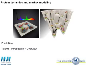
Protein dynamics and Markov modeling: Introduction + Overview - PowerPoint PPT Presentation

Protein dynamics and Markov modeling: Introduction + Overview Fabian Paul Computer Tutorial in Markov Modeling (PyEMMA) Talk 1

Protein 3-D structure and function Proteins are biomolecules that carry out their function via their 3-D • structure, e. g. a receptor binding a molecule to detect a flavor or odor. Which functions? • catalysis gene expression regulation molecular recognition defense proteins information processing … rigidity cellular communication To function, proteins have to change their 3-D structure with time, e. g.: • open ↔ closed (for regulation) • active ↔ inactive (for information processing, communication) • assembled ↔ disassembled (for rigidity+motion), … • 2

Proteins in motion: time and timescales 1s protein folding Met ! -helix 10 -3 s larger Phe domain Asp motion Ala 10 -6 s " -sheet formation Arg of helices, Leu loop 10 -9 s Val motions Gln side-chain rotamers structural 10 -12 s folded structure sequence elements 10 -8 m 10 -10 m bond 10 -15 s vibra3on 3

Molecular dynamics (MD) simulation Experiment cannot resolve all temporal and spatial scales • simultaneously. Experiments either have • high spatial resolution but low temporal resolution (e. g. cryo-electron microscopy*, X-ray diffraction) • high temporal resolution but limited spatial information. (e. g. single molecule fluorescence resonance energy transfer) Molecular dynamics simulation is an important tool that allows to • observe molecules with simultaneously high temporal and high spatial resolution (“virtual microscope”). * Nobel prize in Chemistry 2017 awarded to Dubochet, Frank, and Henderson for cryo-electron microscopy 4

What is molecular dynamics (MD) simulation? Molecular dynamics* uses classical mechanics to model molecular systems and consists of: 1. Equations of motion for the centers of masses ! " of the atoms, e. g. Langevin equations # " ̈ ! " = −'# " ̇ ! " − ) " * ! + , … , ! . + 21 2 3' 4 " 5 with standard normally distributed random variates (7 " ) 9 2. Molecular potential energy model *(!) ”force field” that consists of energy terms for bonded and non-bonded interactions. * Nobel prize in Chemistry 2013 awarded to Karplus, Levitt and Warshel for development of MD 5

Reachable time scales in MD simulation protein 1s unbinding protein folding 10 -3 s larger domain motion 10 -6 s formation of helices, loop 10 -9 s motions side-chain 10 μs / day / Anton I 100 ns / day / GPU* Rate rotamers e.g. Amber, AceMD, OpenMM 10 -12 s bond 10 -15 s vibration 6

Reachable time scales in MD simulation protein 1s unbinding protein folding 10 -3 s larger domain motion 10 -6 s formation of helices, loop 10 -9 s motions side-chain 10 μs / day / Anton I 100 ns / day / GPU* Rate rotamers e.g. Amber, AceMD, OpenMM 10 -12 s 1 Anton I 100 GPUs 1 traj. of 10 μs / day 100 traj. of 100 ns / day Throughput 10 μs / day 10 μs / day bond 10 -15 s vibration 10.000.000 USD Cost 100.000 USD 7

First generation Markov state models (MSMs) 8

Conformational dynamics 9

First generation Markov state models (MSMs) Markov state models (MSMs) can be used as a tool for the systematic • analysis of multiple MD trajectories. A Markov state model consists of: • 1. a set of states ! " "#$,…' 2. (conditional) transition probabilities between these state ( ") = ℙ(! - + / = 0 ∣ !(-) = 3) Unlike MD trajectories, Markov state models are discrete in space • and in time. … 10

First generation Markov state models: estimation Markov model estimation starts with: • grouping of geometrically [1] or kinetically [2] related conformations into clusters or microstates 1 2 microstates 3 [1] Prinz et al ., J. Chem. Phys. 134 , 174105 (2011) [2] Pérez-Hernández, Paul , et al. , J. Chem. Phys. 139 , 015102 (2013) 11

First generation Markov state models: estimation [1] • We then assign every conformation in a MD trajectory to a microstate. !me ! 2 t 3 t 4 t 5 t 6 t 7 t t trajectory microstate " 1 1 2 3 3 2 3 We count transitions between microstates and tabulate them in a • count matrix # e. g. $ %% = 1 , $ %( = 1 , $ () = 2 , … We estimate the transition probabilities + ,- from # . • Naïve estimator: . + ,- = $ ,- / ∑ 1 $ ,1 • ; <= Maximum-likelihood estimator [1]: 2 ∏ ,,- + ,- 3 = argmax • 3 [1] Prinz et al ., J. Chem. Phys. 134 , 174105 (2011) [2] Pérez-Hernández, Paul , et al. , J. Chem. Phys. 139 , 015102 (2013) 12

First generation Markov state models: properties Markov state models: model the probability evolution of an ensemble • p let ! " ($) = ℙ(( $ = )) , then * + ,- = * + 0 / 0 T T T MSMs can extrapolate from the short-time estimate /(-) to long time scales. model the equilibrium distribution of an ensemble • 1 + : = * + ∞ = * + 0 lim 0→8 / 0 MSMs can even extrapolate to infinite time * + ∞ . ( - ≪ ∞ ) We can recover a coarse-grained version of the Boltzmann distribution ( 1 ) without having to estimate / from data distributed according to the Boltzmann distribution. figure adapted from Nüske et al., J. Chem. Theory Comput. 10 , 1739 (2014) 13

Reconciliation with Sampling Problem Analysis Problem Experiment ms - s huge, complex datasets hugedata sets ns - µ s 14

Second generation Markov models: spectral theory time scales: processes: ! " # = ! " 0 & = ' ) ( * ( [, ( ⋅ ! 0 ] ( ! " 1# = ' 2 * ( [, ( ⋅ ! 0 ] ) ( / ( (left) 0 ( (right) ( Eigenfunctions encode the slow relaxation processes. • Eigenfunction point to the location of metastable states. • 15 Prinz et al ., J. Chem. Phys. 134 , 174105 (2011) Sarich et al., SIAM Multiscale Model. Simul . 8 , 1154 (2010). '

Second generation Markov models: variational principle good discretization bad discretization very good discretization If the cluster boundary is misplaced, transition across the • boundary will be faster than transitions over the barrier but never slower . Right eigenfunctions are flat on the metastable states and • change only at/near the barrier. A good discretization allows to represent the eigenfunction well. Equivalence between eigendecomposition and maximizing • “slowness”! 16

Second generation Markov models: variational principle Equivalence between eigendecomposition and maximizing • “slowness”. ' 234 ! = # cov + $ , - , + $ , -/0 ≤ ! ' $%& where + are uncorrelated functions with variance 1. & 5 , … + ' 5 Can maximize the score for multiple functions simultaneously. Variational principle: generate a guess (for the functions) and rank • it with the variational score. The higher, the better. Any algorithm that generates functions which maximize the score • is suitable. Not limited to eigendecompositions / linear algebra. Works in very high-dimensional space. • Result will be close to the true eigenfunctions. • → Approximations will retain properties of the eigenfunctions: encode the slow dynamics, point towards the metastable states. 17

18

Markov modeling workflow Featurization Dim. Reduction Discretization feature selection TICA k-means Discrete VAMP regspace trajs MD data MSM estimation & validation Maximum likelihood (ML) timescales convergence Discrete Markov MSM Bayesian MSM Chapman-Kolmogorov test trajs model ML hidden MSM Bayesian hidden MSM MSM Analysis spectral analysis metastable states with PCCA++ Markov Knowledge stationary properties TPT model kinetic properties Experimental observables uncertainty estimation

Markov modeling workflow: pentapeptide demo 20

Markov modeling workflow Featurization Dim. Reduction Discretization feature selection TICA k-means Discrete VAMP regspace trajs MD data MSM estimation & validation Maximum likelihood (ML) timescales convergence Discrete Markov MSM Bayesian MSM Chapman-Kolmogorov test trajs model ML hidden MSM Bayesian hidden MSM MSM Analysis spectral analysis metastable states with PCCA++ Markov Knowledge stationary properties TPT model kinetic properties Experimental observables uncertainty estimation

Feature selection Select the set of molecular features that gives the most metastable kinetic model (the higher VAMP score, the better). Use cross-validation prevent interpreting noise as a rare event. 22

Markov modeling workflow Featurization Dim. Reduction Discretization feature selection TICA k-means Discrete VAMP regspace trajs MD data MSM estimation & validation Maximum likelihood (ML) timescales convergence Discrete Markov MSM Bayesian MSM Chapman-Kolmogorov test trajs model ML hidden MSM Bayesian hidden MSM MSM Analysis spectral analysis metastable states with PCCA++ Markov Knowledge stationary properties TPT model kinetic properties Experimental observables uncertainty estimation 23

Dimension reduction Find order parameters (“independent components”) that describe the slowest transitions in the MD data. Reduction to two dimensions allows to visualize various functions of the conformational state as 2-D plots, e.g. a histogram samples 24

Dimension reduction Rare events appear clearly in the time series representations of the independent components. 25