PROFIT-MAXIMIZATION TWO-STEP APPROACH For each level of output Q , - - PDF document

▶

Dec 31, 2023 280 likes •340 views

ECO 305 FALL 2003 October 16 PROFIT-MAXIMIZATION TWO-STEP APPROACH For each level of output Q , produce it at minimum cost: min { w L + r K | F ( L, K ) Q ) } Result: conditional input demands L ( w, r, Q ) , K ( w, r, Q )

SLIDE 1

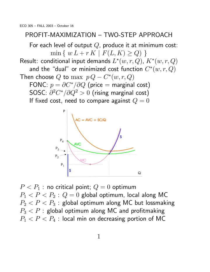
ECO 305 — FALL 2003 — October 16

PROFIT-MAXIMIZATION — TWO-STEP APPROACH For each level of output Q, produce it at minimum cost: min { w L + r K | F(L, K) ≥ Q) } Result: conditional input demands L∗(w, r, Q), K∗(w, r, Q) and the “dual” or minimized cost function C∗(w, r, Q) Then choose Q to max p Q − C∗(w, r, Q) FONC: p = ∂C∗/∂Q (price = marginal cost) SOSC: ∂2C∗/∂Q2 > 0 (rising marginal cost) If fixed cost, need to compare against Q = 0 P < P1 : no critical point; Q = 0 optimum P1 < P < P2 : Q = 0 global optimum, local along MC P2 < P < P3 : global optimum along MC but lossmaking P3 < P : global optimum along MC and profitmaking P1 < P < P4 : local min on decreasing portion of MC 1

SLIDE 2

PROFIT MAXIMIZATION — SINGLE-STEP APPROACH max Π = p F(K, L) − w L − r K FONCs — price of each input = value of its marginal product p ∂F/∂L = w, p ∂F/∂K = r SOSCs — (1) diminishing marginal returns to each input, (2) diminishing returns to scale (this is not fully rigorous) Result - (unconditional) input demand functions L∗(p, w, r), K∗(p, w, r), yielding Q∗ = F(K∗, L∗) Substitute in profit expression to get “dual” profit function Π∗(p, w, r) = p Q∗ − w L∗ − r K∗ Properties of dual profit function: (1) Homogeneous degree 1, and (2) convex in (p, w, r) (3) Hotelling’s lemma: Q∗ = ∂Π∗/∂p, L∗ = − ∂Π∗/∂w, K∗ = − ∂Π∗/∂r Proof of these follows same lines as those of concavity of expenditure functions - take initial (pa, wa, ra) and initially

ptimum La, Ka, Qa. Could go on using these when prices

change, so new optimum choices should yield no less profit. 2

SLIDE 3

EMPIRICAL ESTIMATION U.S. MANUFACTURING (Ernst Berndt, 1991) ln C = ln(α0) +

X

i

αi ln(Pi) +1

2

X

i

X

j

γij ln(Pi) ln(Pj) +αY ln Y + 1

2 γY Y (ln Y )2

+

X

i

γiY ln(Pi) ln Y i, j = inputs K, L, E, and M

X

i

αi = 1, γij = γji,

X

i

γij = 0 Find factor cost share functions and estimate, e.g. PL L C = PL C ∂C ∂PL = d ln C d ln PL . Results: Elasticities of substitution σKL = 0.97, σKE = −3.60, σKM = 0.35, σLM = 0.61, σEM = 0.83, σLE = 0.68 Own price elasticities of factor demands ²K = −0.34, ²L = −0.45, ²E = −0.53, ²M = −0.24 . 3

SLIDE 4

CREDIT UNIONS (Moeller, Princeton Sr Thesis 1999) ln C = a + b1 ln Q + b2 (ln Q)2 +

X

i

ci ln Wi +

X

j

dj ln Fj + µ , where Q = size (output) of the credit union Wi factor prices, Fj other structural variables µ is stochastic error term. Results b1 = 0.6537 with standard error 0.0231, b2 = 0.0204 with standard error 0.0015. b1 < 1, b2 > 0 : initial economies of scale and eventual diseconomies Averge cost is minimized when ln Q = (1 − b1)/(2 b2) = 8.48,