Probabilistic Graphical Models David Sontag New York University - PowerPoint PPT Presentation

Probabilistic Graphical Models David Sontag New York University Lecture 4, February 16, 2012 David Sontag (NYU) Graphical Models Lecture 4, February 16, 2012 1 / 27

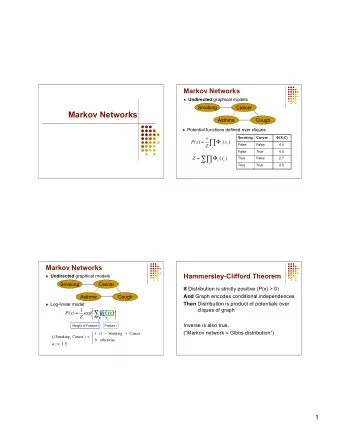
Undirected graphical models Reminder of lecture 2 An alternative representation for joint distributions is as an undirected graphical model (also known as Markov random fields ) As in BNs, we have one node for each random variable Rather than CPDs, we specify (non-negative) potential functions over sets of variables associated with cliques C of the graph, p ( x 1 , . . . , x n ) = 1 � φ c ( x c ) Z c ∈ C Z is the partition function and normalizes the distribution: � � Z = φ c ( ˆ x c ) x 1 ,..., ˆ ˆ x n c ∈ C David Sontag (NYU) Graphical Models Lecture 4, February 16, 2012 2 / 27

Undirected graphical models p ( x 1 , . . . , x n ) = 1 � � � φ c ( x c ) , Z = φ c ( ˆ x c ) Z c ∈ C x 1 ,..., ˆ ˆ x n c ∈ C Simple example (potential function on each edge encourages the variables to take the same value): C C B φ A,B ( a, b ) = φ B,C ( b, c ) = φ A,C ( a, c ) = 0 1 0 1 0 1 B 0 10 1 0 10 1 0 10 1 A B A 1 1 10 1 1 1 10 1 10 A C p ( a , b , c ) = 1 Z φ A , B ( a , b ) · φ B , C ( b , c ) · φ A , C ( a , c ) , where � a , ˆ b ) · φ B , C (ˆ Z = φ A , B (ˆ b , ˆ c ) · φ A , C (ˆ a , ˆ c ) = 2 · 1000 + 6 · 10 = 2060 . a , ˆ ˆ b , ˆ c ∈{ 0 , 1 } 3 David Sontag (NYU) Graphical Models Lecture 4, February 16, 2012 3 / 27

Example: Ising model Theoretical model of interacting atoms, studied in statistical physics and material science Each atom X i ∈ {− 1 , +1 } , whose value is the direction of the atom spin The spin of an atom is biased by the spins of atoms nearby on the material: = +1 = -1 p ( x 1 , · · · , x n ) = 1 � � � � Z exp w i , j x i x j − u i x i i < j i When w i , j > 0, nearby atoms encouraged to have the same spin (called ferromagnetic ), whereas w i , j < 0 encourages X i � = X j Node potentials exp( − u i x i ) encode the bias of the individual atoms Scaling the parameters makes the distribution more or less spiky David Sontag (NYU) Graphical Models Lecture 4, February 16, 2012 4 / 27

Today’s lecture Markov random fields Bayesian networks ⇒ Markov random fields ( moralization ) 1 Hammersley-Clifford theorem (conditional independence ⇒ joint 2 distribution factorization) Conditional models Discriminative versus generative classifiers 3 Conditional random fields 4 David Sontag (NYU) Graphical Models Lecture 4, February 16, 2012 5 / 27

Converting BNs to Markov networks What is the equivalent Markov network for a hidden Markov model? Y5 Y6 Y3 Y4 Y1 Y2 X1 X2 X3 X4 X5 X6 David Sontag (NYU) Graphical Models Lecture 4, February 16, 2012 6 / 27

Moralization of Bayesian networks Procedure for converting a Bayesian network into a Markov network The moral graph M [ G ] of a BN G = ( V , E ) is an undirected graph over V that contains an undirected edge between X i and X j if there is a directed edge between them (in either direction) 1 X i and X j are both parents of the same node 2 A B A B Moralization C D C D (term historically arose from the idea of “marrying the parents” of the node) The addition of the moralizing edges leads to the loss of some independence information, e.g., A → C ← B , where A ⊥ B is lost David Sontag (NYU) Graphical Models Lecture 4, February 16, 2012 7 / 27

Converting BNs to Markov networks Moralize the directed graph to obtain the undirected graphical model: 1 A B A B Moralization C D C D Introduce one potential function for each CPD: 2 φ i ( x i , x pa ( i ) ) = p ( x i | x pa ( i ) ) So, converting a hidden Markov model to a Markov network is simple: David Sontag (NYU) Graphical Models Lecture 4, February 16, 2012 8 / 27

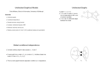
Factorization implies conditional independencies p ( x ) is a Gibbs distribution over G if it can be written as p ( x 1 , . . . , x n ) = 1 � φ c ( x c ) , Z c ∈ C where the variables in each potential c ∈ C form a clique in G Recall that conditional independence is given by graph separation: X B X A X C Theorem ( soundness of separation ): If p ( x ) is a Gibbs distribution for G , then G is an I-map for p ( x ), i.e. I ( G ) ⊆ I ( p ) Proof: Suppose B separates A from C . Then we can write p ( X A , X B , X C ) = 1 Z f ( X A , X B ) g ( X B , X C ) . David Sontag (NYU) Graphical Models Lecture 4, February 16, 2012 9 / 27

Conditional independencies implies factorization Theorem ( soundness of separation ): If p ( x ) is a Gibbs distribution for G , then G is an I-map for p ( x ), i.e. I ( G ) ⊆ I ( p ) What about the converse? We need one more assumption: A distribution is positive if p ( x ) > 0 for all x Theorem ( Hammersley-Clifford , 1971): If p ( x ) is a positive distribution and G is an I-map for p ( x ), then p ( x ) is a Gibbs distribution that factorizes over G Proof is in book (as is counter-example for when p ( x ) is not positive) This is important for learning : Prior knowledge is often in the form of conditional independencies (i.e., a graph structure G ) Hammersley-Clifford tells us that it suffices to search over Gibbs distributions for G – allows us to parameterize the distribution David Sontag (NYU) Graphical Models Lecture 4, February 16, 2012 10 / 27

Today’s lecture Markov random fields Bayesian networks ⇒ Markov random fields ( moralization ) 1 Hammersley-Clifford theorem (conditional independence ⇒ joint 2 distribution factorization) Conditional models Discriminative versus generative classifiers 3 Conditional random fields 4 David Sontag (NYU) Graphical Models Lecture 4, February 16, 2012 11 / 27

Discriminative versus generative classifiers There is often significant flexibility in choosing the structure and parameterization of a graphical model It is important to understand the trade-offs In the next few slides, we will study this question in the context of e-mail classification David Sontag (NYU) Graphical Models Lecture 4, February 16, 2012 12 / 27

From lecture 1 . . . naive Bayes for classification Classify e-mails as spam ( Y = 1) or not spam ( Y = 0) Let 1 : n index the words in our vocabulary (e.g., English) X i = 1 if word i appears in an e-mail, and 0 otherwise E-mails are drawn according to some distribution p ( Y , X 1 , . . . , X n ) Words are conditionally independent given Y : Label Y . . . X1 X2 X3 Xn Features Prediction given by: p ( Y = 1) � n i =1 p ( x i | Y = 1) p ( Y = 1 | x 1 , . . . x n ) = y = { 0 , 1 } p ( Y = y ) � n � i =1 p ( x i | Y = y ) David Sontag (NYU) Graphical Models Lecture 4, February 16, 2012 13 / 27

Discriminative versus generative models Recall that these are equivalent models of p ( Y , X ): Generative Discriminative Y X X Y However, suppose all we need for prediction is p ( Y | X ) In the left model, we need to estimate both p ( Y ) and p ( X | Y ) In the right model, it suffices to estimate just the conditional distribution p ( Y | X ) We never need to estimate p ( X )! Not possible to use this model when X is only partially observed Called a discriminative model because it is only useful for discriminating Y ’s label David Sontag (NYU) Graphical Models Lecture 4, February 16, 2012 14 / 27

Discriminative versus generative models Let’s go a bit deeper to understand what are the trade-offs inherent in each approach Since X is a random vector, for Y → X to be equivalent to X → Y , we must have: Generative Discriminative Y . . . X1 X2 X3 Xn . . . X1 X2 X3 Xn Y We must make the following choices: In the generative model, how do we parameterize p ( X i | X pa ( i ) , Y )? 1 In the discriminative model, how do we parameterize p ( Y | X )? 2 David Sontag (NYU) Graphical Models Lecture 4, February 16, 2012 15 / 27

Discriminative versus generative models We must make the following choices: 1 In the generative model, how do we parameterize p ( X i | X pa ( i ) , Y )? 2 In the discriminative model, how do we parameterize p ( Y | X )? Generative Discriminative Y . . . X1 X2 X3 Xn . . . X1 X2 X3 Xn Y 1 For the generative model, assume that X i ⊥ X − i | Y ( naive Bayes ) 2 For the discriminative model, assume that e α 0 + � n i =1 α i x i 1 p ( Y = 1 | x ; α ) = i =1 α i x i = 1 + e α 0 + � n 1 + e − α 0 − � n i =1 α i x i This is called logistic regression . (To simplify the story, we assume X i ∈ { 0 , 1 } ) David Sontag (NYU) Graphical Models Lecture 4, February 16, 2012 16 / 27

Naive Bayes 1 For the generative model, assume that X i ⊥ X − i | Y ( naive Bayes ) Y Y . . . . . . X1 X2 X3 Xn X1 X2 X3 Xn David Sontag (NYU) Graphical Models Lecture 4, February 16, 2012 17 / 27

Logistic regression 2 For the discriminative model, assume that e α 0 + � n i =1 α i x i 1 p ( Y = 1 | x ; α ) = i =1 α i x i = 1 + e α 0 + � n 1 + e − α 0 − � n i =1 α i x i Let z ( α, x ) = α 0 + � n i =1 α i x i .Then, p ( Y = 1 | x ; α ) = f ( z ( α, x )), where f ( z ) = 1 / (1 + e − z ) is called the logistic function : 1 . . . X1 X2 X3 Xn 1 + e − z Same graphical model Y z David Sontag (NYU) Graphical Models Lecture 4, February 16, 2012 18 / 27