Graphical Models Aarti Singh Slides Courtesy: Carlos Guestrin - PowerPoint PPT Presentation
Graphical Models Aarti Singh Slides Courtesy: Carlos Guestrin Machine Learning 10-701/15-781 Nov 15, 2010 Directed Bayesian Networks Compact representation for a joint probability distribution Bayes Net = Directed Acyclic Graph (DAG)
Graphical Models Aarti Singh Slides Courtesy: Carlos Guestrin Machine Learning 10-701/15-781 Nov 15, 2010
Directed – Bayesian Networks • Compact representation for a joint probability distribution • Bayes Net = Directed Acyclic Graph (DAG) + Conditional Probability Tables (CPTs) • distribution factorizes according to graph ≡ distribution satisfies local Markov independence assumptions ≡ x k is independent of its non-descendants given its parents pa k
Directed – Bayesian Networks • Graph encodes local independence assumptions (local Markov Assumptions) • Other independence assumptions can be read off the graph using d-separation • distribution factorizes according to graph ≡ distribution satisfies all independence assumptions found by d-separation F I • Does the graph capture all independencies? Yes, for almost all distributions that factorize according to graph. More in 10-708
D-separation • a is D-separated from b by c ≡ a b|c • Three important configurations c a … … b c a b Causal direction a b|c Common cause a b|c a b a b V-structure (Explaining away) … a b|c c c
Undirected – Markov Random Fields • Popular in statistical physics, computer vision, sensor networks, social networks, protein-protein interaction network • Example – Image Denoising x i – value at pixel i y i – observed noisy value
Conditional Independence properties • No directed edges • Conditional independence ≡ graph separation • A, B, C – non-intersecting set of nodes • A B|C if all paths between nodes in A & B are “blocked” i.e. path contains a node z in C.
Factorization • Joint distribution factorizes according to the graph Clique, x C = {x 1 ,x 2 } Arbitrary positive function Maximal clique x C = {x 2 ,x 3 ,x 4 } typically NP-hard to compute
MRF Example Often Energy of the clique (e.g. lower if variables in clique take similar values)
MRF Example Ising model: cliques are edges x C = {x i ,x j } binary variables x i ϵ {-1,1} 1 if x i = x j -1 if x i ≠ x j Probability of assignment is higher if neighbors x i and x j are same
Hammersley-Clifford Theorem • Set of distributions that factorize according to the graph - F • Set of distributions that respect conditional independencies implied by graph-separation – I I F Important because: Given independencies of P can get MRF structure G I F Important because: Read independencies of P from MRF structure G
What you should know… • Graphical Models: Directed Bayesian networks, Undirected Markov Random Fields – A compact representation for large probability distributions – Not an algorithm • Representation of a BN, MRF – Variables – Graph – CPTs • Why BNs and MRFs are useful • D-separation (conditional independence) & factorization
Topics in Graphical Models • Representation – Which joint probability distributions does a graphical model represent? • Inference – How to answer questions about the joint probability distribution? • Marginal distribution of a node variable • Most likely assignment of node variables • Learning – How to learn the parameters and structure of a graphical model?
Inference • Possible queries: Flu 1) Marginal distribution e.g. P(S) Allergy Posterior distribution e.g. P(F|H=1) Sinus 2) Most likely assignment of nodes Nose Headache arg max P(F=f,A=a,S=s,N=n|H=1) f,a,s,n
Inference • Possible queries: Flu 1) Marginal distribution e.g. P(S) Allergy Posterior distribution e.g. P(F|H=1) Sinus P(F|H=1) ? P(F, H=1) P(F|H=1) = Nose Headache P(H=1) P(F, H=1) = ∑ P(F= f,H=1) f P(F, H=1) will focus on computing this, posterior will follow with only constant times more effort
Marginalization Need to marginalize over other vars Flu Allergy P(S) = ∑ P( f,a,S,n,h) f,a,n,h Sinus P(F,H=1) = ∑ P( F,a,s,n,H=1) a,s,n 2 3 terms Nose Headache To marginalize out n binary variables, need to sum over 2 n terms Inference seems exponential in number of variables! Actually, inference in graphical models is NP-hard
Bayesian Networks Example • 18 binary attributes • Inference – P(BatteryAge|Starts=f) • need to sum over 2 16 terms! • Not impressed? – HailFinder BN – more than 3 54 = 58149737003040059690 390169 terms
Fast Probabilistic Inference P(F,H=1) = ∑ P( F,a,s,n,H=1) Flu Allergy a,s,n = ∑ P(F)P(a)P( s|F,a)P(n|s)P(H=1|s) a,s,n Sinus = P(F) ∑ P(a) ∑ P( s|F,a )P(H=1|s) ∑ P( n|s) a s n Nose Headache Push sums in as far as possible Distributive property: x 1 z + x 2 z = z(x 1 +x 2 ) 2 multiply 1 mulitply
Fast Probabilistic Inference P(F,H=1) = ∑ P( F,a,s,n,H=1) Flu Allergy a,s,n 8 values x 4 multiplies = ∑ P(F)P(a)P( s|F,a)P(n|s)P(H=1|s) a,s,n 1 Sinus = P(F) ∑ P(a) ∑ P( s|F,a )P(H=1|s) ∑ P( n|s) a s n = P(F) ∑ P(a) ∑ P( s|F,a)P(H=1|s) a s Nose 4 values x 1 multiply Headache = P(F) ∑ P(a) g 1 (F,a) a 32 multiplies vs. 7 multiplies 2 values x 1 multiply 2 n vs. n 2 k = P(F) g 2 (F) k – scope of largest factor 1 multiply (Potential for) exponential reduction in computation!
Fast Probabilistic Inference – Variable Elimination P(F,H=1) = ∑ P(F)P(a)P( s|F,a)P(n|s)P(H=1|s) Flu Allergy a,s,n 1 = P(F) ∑ P(a) ∑ P( s|F,a )P(H=1|s) ∑ P( n|s) a s n Sinus P(H=1|F,a) P(H=1|F) Nose Headache (Potential for) exponential reduction in computation!
Variable Elimination – Order can make a HUGE difference P(F,H=1) = ∑ P(F)P(a)P( s|F,a)P(n|s)P(H=1|s) Flu Allergy a,s,n 1 = P(F) ∑ P(a) ∑ P( s|F,a )P(H=1|s) ∑ P( n|s) a s n Sinus P(H=1|F,a) P(H=1|F) Nose Headache P(F,H=1) = P(F) ∑ P(a) ∑ ∑ P( s|F,a)P(n|s)P(H=1|s) a n s 3 – scope of largest factor g(F,a,n) (Potential for) exponential reduction in computation!
Variable Elimination – Order can make a HUGE difference Y X 1 X 2 X 3 X 4 1 – scope of largest factor g(Y) n – scope of largest factor g(X 1 ,X 2 ,..,X n )
Variable Elimination Algorithm • Given BN – DAG and CPTs (initial factors – p(x i |pa i ) for i=1,..,n) • Given Query P(X|e ) ≡ P( X,e) X – set of variables IMPORTANT!!! • Instantiate evidence e e.g. set H=1 • Choose an ordering on the variables e.g., X 1 , …, X n • For i = 1 to n, If X i {X,e} – Collect factors g 1 ,…, g k that include X i – Generate a new factor by eliminating X i from these factors – Variable X i has been eliminated! – Remove g 1 ,…, g k from set of factors but add g • Normalize P(X,e) to obtain P(X|e)
Complexity for (Poly)tree graphs Variable elimination order: • Consider undirected version • Start from “leaves” up • find topological order • eliminate variables in reverse order Does not create any factors bigger than original CPTs For polytrees, inference is linear in # variables (vs. exponential in general)!
Complexity for graphs with loops • Loop – undirected cycle Linear in # variables but exponential in size of largest factor generated! Moralize graph (connect parents into a clique & drop direction of all edges) When you eliminate a variable, add edges between its neighbors
Complexity for graphs with loops • Loop – undirected cycle Factor generated Var eliminated g 1 (C,B) S g 2 (C,O,D) B D g 3 (C,O) C g 4 (T,O) T g 5 (O,X) O g 6 (X) Linear in # variables but exponential in size of largest factor generated ~ tree-width (max clique size-1) in resulting graph!
Example: Large tree-width with small number of parents At most 2 parents per node, but tree width is O(√n) Compact representation Easy inference
Choosing an elimination order • Choosing best order is NP-complete – Reduction from MAX-Clique • Many good heuristics (some with guarantees) • Ultimately, can’t beat NP -hardness of inference – Even optimal order can lead to exponential variable elimination computation • In practice – Variable elimination often very effective – Many (many many) approximate inference approaches available when variable elimination too expensive
Inference • Possible queries: Flu 2) Most likely assignment of nodes Allergy arg max P(F=f,A=a,S=s,N=n|H=1) f,a,s,n Sinus Use Distributive property: Nose Headache max(x 1 z, x 2 z) = z max(x 1 ,x 2 ) 2 multiply 1 mulitply
Topics in Graphical Models • Representation – Which joint probability distributions does a graphical model represent? • Inference – How to answer questions about the joint probability distribution? • Marginal distribution of a node variable • Most likely assignment of node variables • Learning – How to learn the parameters and structure of a graphical model?
Learning Data CPTs – x (1) … P(X i | Pa Xi ) x (m) structure parameters Given set of m independent samples (assignments of random variables), find the best (most likely?) Bayes Net (graph Structure + CPTs)
Learning the CPTs (given structure) For each discrete variable X k Data Compute MLE or MAP estimates for x (1) … x (m)
MLEs decouple for each CPT in Bayes Nets F A • Given structure, log likelihood of data S N H (j) (j) (j) (j) (j) (j) (j) (j) (j) (j) (j) (j) (j) (j) (j) (j) (j) (j) (j) (j) (j) (j) (j) q F q A q F,A (j) (j) (j)(j) Depends only on q H|S q N|S Can computer MLEs of each parameter independently!
Information theoretic interpretation of MLE Plugging in MLE estimates: ML score Reminds of entropy
Recommend
More recommend
Explore More Topics
Stay informed with curated content and fresh updates.
