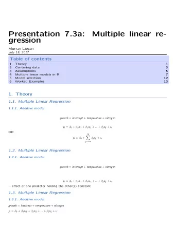
Presentation 7.3b: Multiple linear re- gression Murray Logan - PDF document

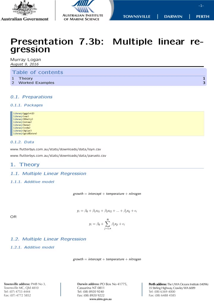
-1- Presentation 7.3b: Multiple linear re- gression Murray Logan August 9, 2016 Table of contents 1 Theory 1 2 Worked Examples 3 0.1. Preparations 0.1.1. Packages library(ggplot2) library(car) library(GGally) library(rstan) library(brms) library(coda) library(dplyr) library(gridExtra) 0.1.2. Data www.flutterbys.com.au/stats/downloads/data/loyn.csv www.flutterbys.com.au/stats/downloads/data/paruelo.csv 1. Theory 1.1. Multiple Linear Regression 1.1.1. Additive model growth = intercept + temperature + nitrogen y i = β 0 + β 1 x i 1 + β 2 x i 2 + ... + β j x ij + ϵ i OR N ∑ y i = β 0 + β j x ji + ϵ i j =1: n 1.2. Multiple Linear Regression 1.2.1. Additive model growth = intercept + temperature + nitrogen

-2- y i = β 0 + β 1 x i 1 + β 2 x i 2 + ... + β j x ij + ϵ i - effect of one predictor holding the other(s) constant 1.3. Multiple Linear Regression 1.3.1. Additive model growth = intercept + temperature + nitrogen y i = β 0 + β 1 x i 1 + β 2 x i 2 + ... + β j x ij + ϵ i Y X1 X2 3 22.7 0.9 2.5 23.7 0.5 6 25.7 0.6 5.5 29.1 0.7 9 22 0.8 8.6 29 1.3 12 29.4 1 1.4. Multiple Linear Regression 1.4.1. Multiplicative model growth = intercept + temp + nitro + temp × nitro y i = β 0 + β 1 x i 1 + β 2 x i 2 + β 3 x i 1 x i 2 + ... + ϵ i 1.5. Assumtions • normality, homogeneity of variance, linearity • (multi)collinearity

-3- 1.6. Multiple Linear Regression 1.6.1. Variance inflation 1 var . inf = 1 − R 2 Collinear when var . inf > = 5 Some prefer > 3 2. Worked Examples 2.1. Worked examples loyn <- read.csv('../data/loyn.csv', strip.white=T) head(loyn) ABUND AREA YR.ISOL DIST LDIST GRAZE ALT 1 5.3 0.1 1968 39 39 2 160 2 2.0 0.5 1920 234 234 5 60 3 1.5 0.5 1900 104 311 5 140 4 17.1 1.0 1966 66 66 3 160 5 13.8 1.0 1918 246 246 5 140 6 14.1 1.0 1965 234 285 3 130 2.2. Worked Examples Question: what effects do fragmentation variables have on the abundance of forest birds Linear model: Abund i ∼ N ( µ , σ 2 ) N ∑ µ = β 0 + β j X ji j =1: n β 0 , β j ∼ N (0, 1000) σ ∼ Cauchy (0, 5)

-4- 2.3. Worked Examples paruelo <- read.csv('../data/paruelo.csv', strip.white=T) head(paruelo) C3 LAT LONG MAP MAT JJAMAP DJFMAP 1 0.65 46.40 119.55 199 12.4 0.12 0.45 2 0.65 47.32 114.27 469 7.5 0.24 0.29 3 0.76 45.78 110.78 536 7.2 0.24 0.20 4 0.75 43.95 101.87 476 8.2 0.35 0.15 5 0.33 46.90 102.82 484 4.8 0.40 0.14 6 0.03 38.87 99.38 623 12.0 0.40 0.11 2.4. Worked Examples Question: what effects do fragmentation geographical variables have on the abundance of C3 grasses Linear model: √ C 3 i ∼ N ( µ , σ 2 ) N ∑ µ = β 0 + β j X ji j =1: n β 0 , β j ∼ N (0, 1000) σ ∼ Cauchy (0, 5)