Multiple Decrement Models Lecture: Weeks 8-9 Lecture: Weeks 8-9 - PowerPoint PPT Presentation

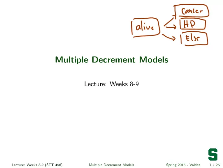
Multiple Decrement Models Lecture: Weeks 8-9 Lecture: Weeks 8-9 (STT 456) Multiple Decrement Models Spring 2015 - Valdez 1 / 25

Multiple decrement models Lecture summary Multiple decrement model - expressed in terms of multiple state model Multiple Decrement Tables (MDT) several causes of decrement probabilities of decrement forces of decrement The Associated Single Decrement Tables (ASDT) Uniform distribution of decrements in the multiple decrement context in the associated single decrement context Chapter 8 (DHW), Sections 8.8-8.12 Lecture: Weeks 8-9 (STT 456) Multiple Decrement Models Spring 2015 - Valdez 2 / 25

Multiple decrement models examples Examples of multiple decrement models Multiple decrement models are extensions of standard mortality models whereby there is simultaneous operation of several causes of decrement. A life fails because of one of these decrements. Examples include: life insurance contract is terminated because of death/survival or withdrawal (lapse). an insurance contract provides coverage for disability and death, which are considered distinct claims. life insurance contract pays a different benefit for different causes of death (e.g. accidental death benefits are doubled). pension plan provides benefit for death, disability, employment termination and retirement. Lecture: Weeks 8-9 (STT 456) Multiple Decrement Models Spring 2015 - Valdez 3 / 25

Multiple decrement models notation Introducing notation age no. of lives heart disease accidents other causes ℓ ( τ ) d (1) d (2) d (3) x x x x x 50 4 , 832 , 555 5 , 168 1 , 157 4 , 293 51 4 , 821 , 927 5 , 363 1 , 206 5 , 162 52 4 , 810 , 206 5 , 618 1 , 443 5 , 960 53 4 , 797 , 185 5 , 929 1 , 679 6 , 840 54 4 , 782 , 727 6 , 277 2 , 152 7 , 631 Conventional notation: ℓ ( τ ) represents the surviving population present at exact age x . x d ( j ) represents the number of lives exiting from the population between x ages x and x + 1 due to decrement j . It is also conventional to denote the total number of exits by all modes between ages x and x + 1 by d ( τ ) i.e. x m � d ( τ ) d ( j ) = x x j =1 where m is the total number of possible decrements, and therefore, d ( τ ) = ℓ ( τ ) − ℓ ( τ ) x +1 . x x Lecture: Weeks 8-9 (STT 456) Multiple Decrement Models Spring 2015 - Valdez 4 / 25

Multiple decrement models probabilities Probabilities of decrement The probability that a life ( x ) will leave the group within one year as a result of decrement j : q ( j ) = d ( j ) x /ℓ ( τ ) x . x The probability that ( x ) will leave the group (regardless of decrement): m m q ( τ ) = d ( τ ) x /ℓ ( τ ) � d ( j ) x /ℓ ( τ ) � q ( j ) = = x . x x x j =1 j =1 The probability that ( x ) will remain in the group for at least one year: = ℓ ( τ ) p ( τ ) = 1 − q ( τ ) x +1 /ℓ ( τ ) = ( ℓ ( τ ) − d ( τ ) x ) /ℓ ( τ ) x . x x x x Lecture: Weeks 8-9 (STT 456) Multiple Decrement Models Spring 2015 - Valdez 5 / 25

Multiple decrement models probabilities - continued We also have the probability of remaining in the group after n years = ℓ ( τ ) · p ( τ ) x +1 · · · p ( τ ) p ( τ ) x + n /ℓ ( τ ) = p ( τ ) x + n − 1 . n x x x and the complement q ( τ ) = 1 − p ( τ ) n x . n x The number of failures due to decrement j over the interval ( x, x + n ] is n − 1 d ( j ) d ( j ) � = x + t . n x t =0 These relationships should be straightforward to follow: d ( j ) ℓ ( τ ) · q ( j ) = n x x n x d ( τ ) ℓ ( τ ) · q ( τ ) = n x x n x Lecture: Weeks 8-9 (STT 456) Multiple Decrement Models Spring 2015 - Valdez 6 / 25

Multiple decrement models MDT Illustration of Multiple Decrement Table Expand Multiple Decrement Table (MDT) into: ℓ ( τ ) d (1) d (2) d (3) q (1) q (2) q (3) q ( τ ) p ( τ ) x x x x x x x x x x 50 4 , 832 , 555 5 , 168 1 , 157 4 , 293 0 . 00107 0 . 00024 0 . 00089 0 . 00220 0 . 99780 51 4 , 821 , 927 5 , 363 1 , 206 5 , 162 0 . 00111 0 . 00025 0 . 00107 0 . 00243 0 . 99757 52 4 , 810 , 206 5 , 618 1 , 443 5 , 960 0 . 00117 0 . 00030 0 . 00124 0 . 00271 0 . 99729 53 4 , 797 , 185 5 , 929 1 , 679 6 , 840 0 . 00124 0 . 00035 0 . 00143 0 . 00301 0 . 99699 54 4 , 782 , 727 6 , 277 2 , 152 7 , 631 0 . 00131 0 . 00045 0 . 00160 0 . 00336 0 . 99664 Lecture: Weeks 8-9 (STT 456) Multiple Decrement Models Spring 2015 - Valdez 7 / 25

Multiple decrement models illustrative problems Illustrative problems Using the previously given multiple decrement table, compute and interpret the following: d (3) 1 2 51 p ( τ ) 2 3 50 q (1) 3 2 53 q (2) 4 2 | 2 50 Lecture: Weeks 8-9 (STT 456) Multiple Decrement Models Spring 2015 - Valdez 8 / 25

The continuous case force of decrement Total force of decrement The total force of decrement at age x is defined as 1 = − 1 d = − d h q ( τ ) µ ( τ ) dxℓ ( τ ) dx log ℓ ( τ ) = lim x x x h x ℓ ( τ ) h → 0 x Therefore, analogous to the single decrement table, we have �� t � p ( τ ) µ ( τ ) = exp − x + s ds t x 0 and � 1 s x µ ( τ ) q ( τ ) p ( τ ) = x + s ds x 0 or, more generally � t q ( τ ) s x µ ( τ ) p ( τ ) = x + s ds. t x 0 Lecture: Weeks 8-9 (STT 456) Multiple Decrement Models Spring 2015 - Valdez 9 / 25

The continuous case force of single decrement Force of a single decrement The force of decrement due to decrement j is defined as: = − 1 d µ ( j ) dxℓ ( j ) x . x ℓ ( τ ) x Notice that the denominator is NOT ℓ ( j ) but is rather ℓ ( τ ) x . x As a consequence, we see that m µ ( τ ) � µ ( j ) = x . x j =1 The total force of decrement is (indeed) the sum of all the other partial forces of decrement. We can also show that � 1 s x µ ( j ) q ( j ) p ( τ ) = x + s ds. x 0 Lecture: Weeks 8-9 (STT 456) Multiple Decrement Models Spring 2015 - Valdez 10 / 25

The continuous case illustrative exercise Illustrative exercise Suppose that in a triple-decrement model, you are given constant forces of decrement, for a person now age x , as follows: µ (1) = b , for t ≥ 0 , x + t µ (2) = b , for t ≥ 0 , x + t µ (3) = 2 b , for t ≥ 0 . x + t You are also given that the probability ( x ) will exit the group within 3 years due to decrement 1 is 0.00884. Compute the length of time a person now age x is expected to remain in the triple decrement table. Answer (to be discussed in lecture): 83 1 / 3 years. Lecture: Weeks 8-9 (STT 456) Multiple Decrement Models Spring 2015 - Valdez 11 / 25

The ASDT The associated single-decrement table (ASDT) For each of the causes of decrement in an MDT, a single-decrement table can be defined showing the operation of that decrement independent of the others. called the associated single-decrement table (ASDT) Each table represents a group of lives reduced continuously by only one decrement. For example, a group subject only to death, but not to other decrements such as withdrawal. The associated probabilities in the ASDT are called absolute rates of decrements. For example, the absolute rate of decrement due to decrement j over the interval ( x, x + t ] is q ′ ( j ) . t x One should be able to explain intuitively why the following always hold true: q ′ ( j ) ≥ q ( j ) t x . t x Lecture: Weeks 8-9 (STT 456) Multiple Decrement Models Spring 2015 - Valdez 12 / 25

Link between the MDT and the ASDT Link between the MDT and the ASDT If given the absolute rates of decrements, say q ′ (1) , q ′ (2) , . . . , q ′ ( m ) , x x x how do we derive the probabilities of decrements q (1) x , q (2) x , . . . , q ( m ) in x the MDT? And vice versa. The fundamental link: µ ( j ) = µ ′ ( j ) for all j = 1 , 2 , ..., m . x x Therefore, it follows that p ( τ ) = p ′ (1) × p ′ (2) × · · · × p ′ ( m ) . t x t x t x t x Furthermore, we note that � t q ( j ) · µ ( j ) p ( τ ) = x + s ds t x s x 0 � t � t p ( τ ) · µ ′ ( j ) s x · µ ′ ( j ) p ( τ ) p ′ ( j ) = x + s ds = x + s ds. s x s x p ′ ( j ) 0 0 s x Lecture: Weeks 8-9 (STT 456) Multiple Decrement Models Spring 2015 - Valdez 13 / 25

Link between the MDT and the ASDT In the multiple decrement context We assume the following UDD assumption: q ( j ) = t · q ( j ) x , for 0 ≤ t ≤ 1 . t x This leads us to the following result: x ) q ( j ) x /q ( τ ) p ′ ( j ) x . = (1 − t · q ( τ ) t x Proof to be done in class. This result allows us to compute the absolute rates of decrements q ′ ( j ) given the probabilities of decrements in the multiple decrement x model. In particular, when t = 1 , we have x ) q ( j ) x /q ( τ ) x . q ′ ( j ) = 1 − (1 − q ( τ ) x Lecture: Weeks 8-9 (STT 456) Multiple Decrement Models Spring 2015 - Valdez 14 / 25

Link between the MDT and the ASDT Illustrative example In a double decrement table where cause d is death and cause w is withdrawal, you are given: both deaths and withdrawals are each uniformly distributed over each year of age in the double decrement table. ℓ ( τ ) = 1000 x q ( w ) = 0 . 48 x d ( d ) = 0 . 35 d ( w ) x x Calculate q ′ ( d ) and q ′ ( w ) . x x Note: One way to check your results make sense is to ensure the inequality q ′ ( j ) ≥ q ( j ) is satisfied. x x Lecture: Weeks 8-9 (STT 456) Multiple Decrement Models Spring 2015 - Valdez 15 / 25