On the Metric-based Approximate Minimization of Markov Chains* - PowerPoint PPT Presentation

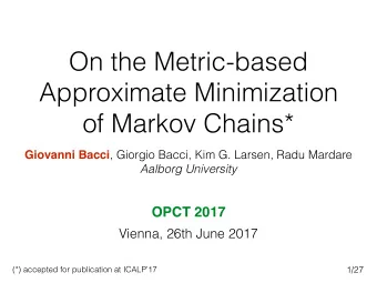
On the Metric-based Approximate Minimization of Markov Chains* Giovanni Bacci, Giorgio Bacci , Kim G. Larsen, Radu Mardare Aalborg University REPAS Meeting Ljubljana, 13th June 2017 (*) accepted for publication at ICALP’17 1/33

Introduction • Moore‘56, Hopcroft‘71: Minimization algorithm for DFA ( partition refinement wrt Myhill-Nerode equiv. ) • Minimization via partition refinement: • Kanellakis-Smolka’83: minimization of LTSs wrt Milner’s strong bisimulation • Baier’96: minimization of MCs wrt Larsen-Skou probabilistic bisimulation • Alur et al.’92, Yannakakis-Lee’97: minimization of timed & real-time transition systems. • and many more… 2/33

A fundamental problem Jou-Smolka’90 observed that behavioral equivalences are not robust for systems with real-valued data ≁ n 0 m 0 1/3 1/3+ ε 1/3 2/3 1/3- ε 1 n 2 n 1 m 1 m 2 1 1 1 n 3 1 3/33

A fundamental problem Jou-Smolka’90 observed that behavioral equivalences are not robust for systems with real-valued data S o l u t i o n ! e q u i v . d i s t a n c e ≁ � d(m 0 ,n 0 ) n 0 m 0 1/3 1/3+ ε 1/3 2/3 1/3- ε 1 n 2 n 1 m 1 m 2 1 1 1 n 3 1 3/33

Metric-based Approximate Minimization Closest Bounded Minimum Significant Approximant (CBA) Approximant Bound (MSAB) 4/33

Metric-based Approximate Minimization Closest Bounded Minimum Significant Approximant (CBA) Approximant Bound (MSAB) MC MC(k) d M N 4/33

Metric-based Approximate Minimization Closest Bounded Minimum Significant Approximant (CBA) Approximant Bound (MSAB) MC MC(k) d M N minimize d 4/33

Metric-based Approximate Minimization Closest Bounded Minimum Significant Approximant (CBA) Approximant Bound (MSAB) MC MC MC(k) MC( k ) d < 1 M M N N minimize d 4/33

Metric-based Approximate Minimization Closest Bounded Minimum Significant Approximant (CBA) Approximant Bound (MSAB) MC MC MC(k) MC( k ) d < 1 M M N N minimize d minimize k 4/33

CBA: Example* 1/2 m 0 1/6 1/3 m 1 m 2 1/2 1/2 1/2 1/2 m 4 1 m 5 m 3 1 1 MC(5) (*) With respect to the undiscounted 5/33 probabilistic bisimilarity distance

CBA: Example* m 0 4/9 1/2 1/2 1/2 m 0 m 12 1/6 1/3 1/6 1/3 1/2 m 1 m 2 m 5 m 4 m 3 1/2 1/2 1 1 1/2 1/2 1 m 4 1 m 5 m 3 1 1 MC(5) (*) With respect to the undiscounted 5/33 probabilistic bisimilarity distance

CBA: Example* m 0 4/9 1/2 1/2 1/2 m 0 m 12 1/6 1/3 1/6 1/6 1/3 1/2 m 1 m 2 m 5 m 4 m 3 1/2 1/2 1 1 1/2 1/2 1 m 0 1/2 m 4 1/3 1/6 1 m 5 m 3 1 m 12 m 12 1 MC(5) 1/2 1/2 1 m 5 m 4 1 1 (*) With respect to the undiscounted 5/33 probabilistic bisimilarity distance

CBA: Example* m 0 4/9 1/2 1/2 1/2 m 0 m 12 1/6 1/3 1/6 1/6 1/3 1/2 m 1 m 2 m 5 m 4 m 3 1/2 1/2 1 1 1/2 1/2 1 m 0 1/2 m 4 1/3 1/6 1 m 5 m 3 1 m 12 m 12 1 MC(5) No unique solution! 1/2 1/2 1 m 5 m 4 1 1 (*) With respect to the undiscounted 5/33 probabilistic bisimilarity distance

CBA: Example* x 79/100 79/100 m 0 m 1 m 3 n 0 1 - x - y 21/100 21/100 79/100 y m 2 m 4 21/100 n 2 n 1 1 1 1 1 6/33 (*) With respect to the undiscounted probabilistic bisimilarity distance

CBA: Example* x 79/100 79/100 m 0 m 1 m 3 n 0 1 - x - y 21/100 21/100 79/100 y m 2 m 4 21/100 n 2 n 1 1 s r 1 e t e m a r a p a l m i t p O ! a l n 1 o t i a r r i e b 1 y a m x = 1 ⇣ ⌘ √ 10 + 163 30 y = 21 200 6/33 (*) With respect to the undiscounted probabilistic bisimilarity distance

CBA: Example* x 79/100 79/100 m 0 m 1 m 3 n 0 1 - x - y 21/100 21/100 79/100 y m 2 m 4 21/100 n 2 n 1 1 s r 1 e t e m a r e a c p n a l a m t s i d i t p l O a m i t p O ! a l n 1 o t i a r r i ! e l b a 1 n y o a i m t a r i r s i √ x = 1 ⇣ ⌘ √ δ ( m 0 , n 0 ) = 436 675 − 163 163 10 + 163 ≈ 0 . 49 30 13500 y = 21 200 6/33 (*) With respect to the undiscounted probabilistic bisimilarity distance

Talk Outline � Probabilistic bisimilarity distance • fixed point characterization (Kantorovich oper.) • remarkable properties • relation with probabilistic model checking � Metric-based Optimal Approximate Minimization • Closest Bounded Approximant (CBA) 
 — definition, characterization, complexity • Minimum Significant Approximant Bound (MSAB) 
 — definition, characterization, complexity • Expectation Maximization-like algorithm 
 — 2 heuristics + experimental results 7/33

Probabilistic bisimulation 1 1 n 1 1/3 m 1 1/3 m 0 n 0 n 2 1/3 1 1 2/3 m 2 1/3 n 3 1 It tries to match the behaviors “quantitatively” 8/33

Probabilistic bisimulation 1 1 1/3 n 1 1/3 m 1 1/3 m 0 n 0 n 2 1/3 1 1 2/3 m 2 1/3 n 3 1 It tries to match the behaviors “quantitatively” 8/33

Probabilistic bisimulation 1 1 1/3 n 1 1/3 m 1 1/3 m 0 n 0 n 2 1/3 1/3 1 1 2/3 m 2 1/3 n 3 1 It tries to match the behaviors “quantitatively” 8/33

Probabilistic bisimulation 1 1 1/3 n 1 1/3 m 1 1/3 m 0 n 0 n 2 1/3 1/3 1 1 2/3 m 2 1/3 n 3 1 1/3 It tries to match the behaviors “quantitatively” 8/33

Coupling Definition (W. Doeblin 36) A coupling of a pair ( μ , ν ) of probability distributions on M is a distribution ω on M × M such that • ∑ n ∈ M ω (m,n) = μ (m) (left marginal) • ∑ m ∈ M ω (m,n) = ν (n) (right marginal) . One can think of a coupling as a measure-theoretic relation between probability distribution 9/33

A quantitative generalization 1 1 1/3 n 1 1/3+ ε m 1 1/3 ε m 0 n 0 n 2 1/3- ε 1/3- ε 1 1 2/3 m 2 1/3 n 3 1/3 1 minimize ∑ ω (u,v) d(u,v) u,v ∈ M 10/33

A quantitative generalization of probabilistic bisimilarity The λ -discounted probabilistic bisimilarity pseudometric is the smallest d λ : M × M → [0,1] such that 1 if ℓ (m) ≠ℓ (n) d λ (m,n) = min λ ∑ ω (u,v) d λ (u,v) otherwise ω ∈ Ω ( τ (m), τ (n)) u,v ∈ M 11/33

A quantitative generalization of probabilistic bisimilarity The λ -discounted probabilistic bisimilarity pseudometric is the smallest d λ : M × M → [0,1] such that 1 if ℓ (m) ≠ℓ (n) d λ (m,n) = min λ ∑ ω (u,v) d λ (u,v) otherwise ω ∈ Ω ( τ (m), τ (n)) u,v ∈ M Kantorovich distance K(d)( μ , ν ) = min ∑ ω (u,v) d(u,v) ω ∈ Ω ( μ , ν ) u,v ∈ M 11/33

Remarkable properties Theorem (Desharnais et. al 99) m ~ n iff d λ (m,n) = 0 Theorem (Chen, van Breugel, Worrell 12) The probabilistic bisimilarity distance can be computed in polynomial time 12/33

Relation with Model Checking Theorem (Chen, van Breugel, Worrell 12) For all φ ∈ LTL | Pr(m ⊨ φ ) - Pr(n ⊨ φ ) | ≤ d 1 (m,n) 13/33

Relation with Model Checking Theorem (Chen, van Breugel, Worrell 12) For all φ ∈ LTL | Pr(m ⊨ φ ) - Pr(n ⊨ φ ) | ≤ d 1 (m,n) …imagine that |M| ≫ |N|, we can use N in place of M approximate Pr( n ⊨ φ ) solution on φ d d 0 1 Pr( m ⊨ φ ) 13/33

Talk Outline � Probabilistic bisimilarity distance • fixed point characterization (Kantorovich oper.) • remarkable properties • relation with probabilistic model checking � Metric-based Optimal Approximate Minimization • Closest Bounded Approximant (CBA) 
 — definition, characterization, complexity • Minimum Significant Approximant Bound (MSAB) 
 — definition, characterization, complexity • Expectation Maximization-like algorithm 
 — 2 heuristics + experimental results 14/33

The CBA- λ problem The Closest Bounded Approximant wrt d λ Instance: An MC M, and a positive integer k Ouput: An MC Ñ, with at most k states minimizing d λ (m 0 ,ñ 0 ) d λ (m 0 ,ñ 0 ) = inf { d λ (m 0 ,n 0 ) | N ∈ MC(k) } we get a solution iff the infimum is a minimum 15/33

The CBA- λ problem The Closest Bounded Approximant wrt d λ Instance: An MC M, and a positive integer k Ouput: An MC Ñ, with at most k states minimizing d λ (m 0 ,ñ 0 ) d λ (m 0 ,ñ 0 ) = inf { d λ (m 0 ,n 0 ) | N ∈ MC(k) } generalization of we get a solution iff the bisimilarity quotient infimum is a minimum 15/33

CBA- λ as a Bilinear Program d λ (m 0 ,ñ 0 ) = inf { d λ (m 0 ,n 0 ) | N ∈ MC(k) } = inf { d(m 0 ,n 0 ) | Γ λ (d) ≤ d, N ∈ MC(k)} 16/33

CBA- λ as a Bilinear Program d λ (m 0 ,ñ 0 ) = inf { d λ (m 0 ,n 0 ) | N ∈ MC(k) } = inf { d(m 0 ,n 0 ) | Γ λ (d) ≤ d, N ∈ MC(k)} mimimize d m 0 ,n 0 such that d m,n = 1 ` ( m ) 6 = ↵ ( n ) ( u,v ) ∈ M × N c m,n � P ` ( m ) = ↵ ( n ) u,v · d u,v  d m,n v ∈ N c m,n P u,v = ⌧ ( m )( u ) m, u 2 M , n 2 N u ∈ M c m,n P u,v = ✓ n,v m 2 M , n, v 2 N c m,n u,v � 0 m, u 2 M , n, v 2 N 16/33

CBA- λ as a Bilinear Program d λ (m 0 ,ñ 0 ) = inf { d λ (m 0 ,n 0 ) | N ∈ MC(k) } = inf { d(m 0 ,n 0 ) | Γ λ (d) ≤ d, N ∈ MC(k)} mimimize d m 0 ,n 0 such that d m,n = 1 ` ( m ) 6 = ↵ ( n ) ( u,v ) ∈ M × N c m,n � P ` ( m ) = ↵ ( n ) u,v · d u,v  d m,n v ∈ N c m,n P u,v = ⌧ ( m )( u ) m, u 2 M , n 2 N u ∈ M c m,n P u,v = ✓ n,v m 2 M , n, v 2 N c m,n u,v � 0 m, u 2 M , n, v 2 N 16/33