Quantum and Classical Algorithms for Approximate Submodular Function - PowerPoint PPT Presentation

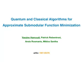
Quantum and Classical Algorithms for Approximate Submodular Function Minimization Yassine Hamoudi, Patrick Rebentrost, Ansis Rosmanis, Miklos Santha arXiv: 1907.05378

1. Approximate Submodular Function Minimization 2. Quantum speed-up for Importance Sampling

1 Approximate Submodular Function Minimization

Submodular Function 4 F : 2 [ n ] → ℝ A submodular function is a set function satisfying the diminishing returns property : ∀ A ⊂ B ⊂ [ n ] and i ∉ B , F ( A ∪ { i }) − F ( A ) ≥ F ( B ∪ { i }) − F ( B )

Submodular Function 4 F : 2 [ n ] → ℝ A submodular function is a set function satisfying the diminishing returns property : ∀ A ⊂ B ⊂ [ n ] and i ∉ B , F ( A ∪ { i }) − F ( A ) ≥ F ( B ∪ { i }) − F ( B ) Example: area covered by cameras A B

Submodular Function 4 F : 2 [ n ] → ℝ A submodular function is a set function satisfying the diminishing returns property : ∀ A ⊂ B ⊂ [ n ] and i ∉ B , F ( A ∪ { i }) − F ( A ) ≥ F ( B ∪ { i }) − F ( B ) Example: area covered by cameras A + i B + i

Submodular Function 5 F : 2 [ n ] → ℝ A submodular function is a set function satisfying the diminishing returns property : ∀ A ⊂ B ⊂ [ n ] and i ∉ B , F ( A ∪ { i }) − F ( A ) ≥ F ( B ∪ { i }) − F ( B ) Example: size of a cut |cut( A )| = 2 B |cut( B )| = 5 A

Submodular Function 5 F : 2 [ n ] → ℝ A submodular function is a set function satisfying the diminishing returns property : ∀ A ⊂ B ⊂ [ n ] and i ∉ B , F ( A ∪ { i }) − F ( A ) ≥ F ( B ∪ { i }) − F ( B ) Example: size of a cut |cut( A )| = 2 B |cut( B )| = 5 A |cut( A + i )| = 4 |cut( B + i )| = 6 i

Submodular Function Minimization 6 Evaluation oracle access: given S obtain F(S) . ( time = #queries to the oracle )

Submodular Function Minimization 6 Evaluation oracle access: given S obtain F(S) . ( time = #queries to the oracle ) Submodular functions can be minimized in polynomial time (Grotschel, Lovasz, Shrijver 1981)

Submodular Function Minimization 6 Evaluation oracle access: given S obtain F(S) . ( time = #queries to the oracle ) Submodular functions can be minimized in polynomial time (Grotschel, Lovasz, Shrijver 1981) Exact Minimization: S ⋆ F ( S ⋆ ) = min find such that S ⊂ [ n ] F ( S ) O ( n 2 log M ) • ˜ ˜ O ( n 3 ) Lee, Sidford, Wong FOCS’15: or where M = max | F ( S ) |

Submodular Function Minimization 6 Evaluation oracle access: given S obtain F(S) . ( time = #queries to the oracle ) Submodular functions can be minimized in polynomial time (Grotschel, Lovasz, Shrijver 1981) Exact Minimization: S ⋆ F ( S ⋆ ) = min find such that S ⊂ [ n ] F ( S ) O ( n 2 log M ) • ˜ ˜ O ( n 3 ) Lee, Sidford, Wong FOCS’15: or where M = max | F ( S ) | ε -Approx. Minimization: S ⋆ F ( S ⋆ ) ≤ min find such that S ⊂ [ n ] F ( S ) + ϵ ( F : 2 [ n ] → [ − 1,1] )

Submodular Function Minimization 6 Evaluation oracle access: given S obtain F(S) . ( time = #queries to the oracle ) Submodular functions can be minimized in polynomial time (Grotschel, Lovasz, Shrijver 1981) Exact Minimization: S ⋆ F ( S ⋆ ) = min find such that S ⊂ [ n ] F ( S ) O ( n 2 log M ) • ˜ ˜ O ( n 3 ) Lee, Sidford, Wong FOCS’15: or where M = max | F ( S ) | ε -Approx. Minimization: S ⋆ F ( S ⋆ ) ≤ min find such that S ⊂ [ n ] F ( S ) + ϵ ( F : 2 [ n ] → [ − 1,1] ) • Previous work: ˜ O ( n 5/3 / ϵ 2 ) (classical) (Chakrabarty, Lee, Sidford, Wong STOC’17)

Submodular Function Minimization 6 Evaluation oracle access: given S obtain F(S) . ( time = #queries to the oracle ) Submodular functions can be minimized in polynomial time (Grotschel, Lovasz, Shrijver 1981) Exact Minimization: S ⋆ F ( S ⋆ ) = min find such that S ⊂ [ n ] F ( S ) O ( n 2 log M ) • ˜ ˜ O ( n 3 ) Lee, Sidford, Wong FOCS’15: or where M = max | F ( S ) | ε -Approx. Minimization: S ⋆ F ( S ⋆ ) ≤ min find such that S ⊂ [ n ] F ( S ) + ϵ ( F : 2 [ n ] → [ − 1,1] ) • Previous work: ˜ O ( n 5/3 / ϵ 2 ) (classical) (Chakrabarty, Lee, Sidford, Wong STOC’17) • Our result: ˜ ˜ O ( n 3/2 / ϵ 2 ) O ( n 5/4 / ϵ 5/2 ) or (classical) (quantum)

Lovász Extension 7 Discrete Optimization F : 2 [ n ] → ℝ Set function:

Lovász Extension 7 Discrete Optimization F : 2 [ n ] → ℝ Set function: Continuous Optimization f : [0,1] n → ℝ Lovász extension:

Lovász Extension 7 Discrete Optimization F : 2 [ n ] → ℝ Set function: Continuous Optimization f : [0,1] n → ℝ Lovász extension: n = 2 F (Ø) = 0 F ({1}) = 10 F ({2}) = 6 F ({1,2}) = 3

Lovász Extension 7 Discrete Optimization F : 2 [ n ] → ℝ Set function: Continuous Optimization f : [0,1] n → ℝ Lovász extension: n = 2 (1,1) F (Ø) = 0 F ({1}) = 10 F ({2}) = 6 (1,0) (0,1) F ({1,2}) = 3 [0,1] 2 (0,0)

Lovász Extension 7 Discrete Optimization F : 2 [ n ] → ℝ Set function: Continuous Optimization f : [0,1] n → ℝ Lovász extension: F ({1}) F ({1,2}) n = 2 F ({2}) (1,1) F (Ø) = 0 F ({1}) = 10 F ({2}) = 6 (1,0) (0,1) F ({1,2}) = 3 F (Ø) (0,0)

Lovász Extension 7 Discrete Optimization F : 2 [ n ] → ℝ Set function: Continuous Optimization f : [0,1] n → ℝ Lovász extension: F ({1}) F ({1,2}) n = 2 F ({2}) (1,1) F (Ø) = 0 F ({1}) = 10 F ({2}) = 6 (1,0) (0,1) F ({1,2}) = 3 F (Ø) (0,0)

Lovász Extension 8 Discrete Optimization F : 2 [ n ] → ℝ Set function: Continuous Optimization f : [0,1] n → ℝ Lovász extension: F ({1}) The Lovász extension is: F ({1,2}) F ({2}) (1,1) (1,0) (0,1) F (Ø) (0,0)

Lovász Extension 8 Discrete Optimization F : 2 [ n ] → ℝ Set function: Continuous Optimization f : [0,1] n → ℝ Lovász extension: F ({1}) The Lovász extension is: F ({1,2}) F ({2}) (1,1) • Piecewise linear (1,0) (0,1) F (Ø) (0,0)

Lovász Extension 8 Discrete Optimization F : 2 [ n ] → ℝ Set function: Continuous Optimization f : [0,1] n → ℝ Lovász extension: F ({1}) The Lovász extension is: F ({1,2}) F ({2}) (1,1) • Piecewise linear • Convex i ff F is submodular (Lovász 1983) (1,0) (0,1) F (Ø) (0,0)

Lovász Extension 8 Discrete Optimization F : 2 [ n ] → ℝ Set function: Continuous Optimization f : [0,1] n → ℝ Lovász extension: F ({1}) The Lovász extension is: F ({1,2}) F ({2}) (1,1) • Piecewise linear • Convex i ff F is submodular (Lovász 1983) (1,0) (0,1) • Evaluable using n queries to F . F (Ø) (0,0)

Stochastic Subgradient Descent 9 Convex function f : C → ℝ on a convex set C . (not necessarily di ff erentiable)

Stochastic Subgradient Descent 9 Convex function f : C → ℝ on a convex set C . (not necessarily di ff erentiable) Subgradient at x : slope g(x) of any line that is below the graph of f and intersects it at x . g ( x ) f ( x ) x

Stochastic Subgradient Descent 9 Convex function f : C → ℝ on a convex set C . (not necessarily di ff erentiable) Subgradient at x : slope g(x) of any line that is below the graph of f and intersects it at x . g ( x ) f ( x ) x

Stochastic Subgradient Descent 9 Convex function f : C → ℝ on a convex set C . (not necessarily di ff erentiable) Subgradient at x : slope g(x) of any line that is below the graph of f and intersects it at x . Stochastic Subgradient at x : random variable satisfying g ( x ) ˜ E [˜ g ( x )] = g ( x ) g ( x ) w.p. 1/2 ˜ g ( x ) f ( x ) g ( x ) w.p. 1/2 ˜ x

Stochastic Subgradient Descent 10 Convex function f : C → ℝ on a convex set C . (not necessarily di ff erentiable) Subgradient at x : slope g(x) of any line that is below the graph of f and intersects it at x . Stochastic Subgradient at x : random variable satisfying g ( x ) ˜ E [˜ g ( x )] = g ( x ) (projected) Stochastic Subgradient Descent

Stochastic Subgradient Descent 10 Convex function f : C → ℝ on a convex set C . (not necessarily di ff erentiable) Subgradient at x : slope g(x) of any line that is below the graph of f and intersects it at x . Stochastic Subgradient at x : random variable satisfying g ( x ) ˜ E [˜ g ( x )] = g ( x ) (projected) Stochastic Subgradient Descent x t C

Stochastic Subgradient Descent 10 Convex function f : C → ℝ on a convex set C . (not necessarily di ff erentiable) Subgradient at x : slope g(x) of any line that is below the graph of f and intersects it at x . Stochastic Subgradient at x : random variable satisfying g ( x ) ˜ E [˜ g ( x )] = g ( x ) (projected) Stochastic Subgradient Descent x t − η ˜ g ( x t ) C

Stochastic Subgradient Descent 10 Convex function f : C → ℝ on a convex set C . (not necessarily di ff erentiable) Subgradient at x : slope g(x) of any line that is below the graph of f and intersects it at x . Stochastic Subgradient at x : random variable satisfying g ( x ) ˜ E [˜ g ( x )] = g ( x ) (projected) Stochastic Subgradient Descent x t − η ˜ g ( x t ) projection x t +1 C