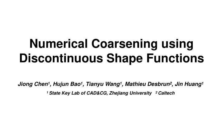
Numerical Coarsening using Discontinuous Shape Functions Jiong Chen - PowerPoint PPT Presentation
Numerical Coarsening using Discontinuous Shape Functions Jiong Chen 1 , Hujun Bao 1 , Tianyu Wang 1 , Mathieu Desbrun 2 , Jin Huang 1 1 State Key Lab of CAD&CG, Zhejiang University 2 Caltech Challenge nonlinear Inhomogeneous Challenge
Numerical Coarsening using Discontinuous Shape Functions Jiong Chen 1 , Hujun Bao 1 , Tianyu Wang 1 , Mathieu Desbrun 2 , Jin Huang 1 1 State Key Lab of CAD&CG, Zhejiang University 2 Caltech
Challenge
nonlinear Inhomogeneous Challenge
Inhomogeneous nonlinear Challenge Require fine mesh
Coarse mesh Inhomogeneous nonlinear Challenge Require fine mesh
Coarse mesh Inhomogeneous nonlinear linear bases Challenge Require fine mesh
Coarse mesh Inhomogeneous nonlinear linear bases Challenge Require fine mesh
Previous works [Nesme 2009] [Kharevych 2009] [Torres 2016]
Not applicable for nonlinear elasticity Previous works [Nesme 2009] [Kharevych 2009] [Torres 2016]
Previous work Data-driven approach to regress the coarse elastic model [Chen 2015]
Rely on data set and parameter tunning Previous work Data-driven approach to regress the coarse elastic model [Chen 2015]
Our solution Z E [ u ] = Ψ ( r u ) dX Ω
Our solution X Z r u = r N i ( X ) u i E [ u ] = Ψ ( r u ) dX i Ω
Our solution X Z r u = r N i ( X ) u i E [ u ] = Ψ ( r u ) dX i Ω i : ∂ 2 Ψ Z r N T K ij ( u ) = ∂ r u 2 : r N j
Our solution X Z r u = r N i ( X ) u i E [ u ] = Ψ ( r u ) dX i Ω
Our solution X Z r u = r N i ( X ) u i E [ u ] = Ψ ( r u ) dX i Ω Homogenize the constitutive model
Our solution X Z r u = r N i ( X ) u i E [ u ] = Ψ ( r u ) dX i Ω Homogenize the constitutive model Approximate the solution space better
Our solution scalar basis 0 0 N(X) ∼ 0 0 • Matrix-valued shape functions = 0 0
Our solution generalize 0 0 N(X) ∼ 0 0 • Matrix-valued shape functions = 0 0 N H : Ω → R d × d i
Our solution generalize 0 0 N(X) ∼ 0 0 • Matrix-valued shape functions = 0 0 N H : Ω → R d × d i • Geometric & physical conditions
Our solution generalize 0 0 N(X) ∼ 0 0 • Matrix-valued shape functions = 0 0 N H : Ω → R d × d i • Geometric & physical conditions Inter-element Inner-element continuity stiffness
Matrix-valued shape function u H u H 3 2 X H X H u H 3 2 1 • Element-wise interpolation u ( X ) u H X 4 X ∀ X ∈ Ω H , u ( X ) = N H i ( X ) u X X H X H i Ω H 4 1 X i ∈ Ω H
Matrix-valued shape function u H u H 3 2 X H X H u H 3 2 1 • Element-wise interpolation u ( X ) u H X 4 X ∀ X ∈ Ω H , u ( X ) = N H i ( X ) u X X H X H i Ω H 4 1 X i ∈ Ω H • Corotational formulation " # i ( X )( R T x H X N H i − X H u ( X ) = R X + i ) − X i
Matrix-valued shape function u H u H 3 2 X H X H u H 3 2 1 • Element-wise interpolation u ( X ) u H X 4 X ∀ X ∈ Ω H , u ( X ) = N H i ( X ) u X X H X H i Ω H 4 1 X i ∈ Ω H • Corotational formulation " # i ( X )( R T x H X N H i − X H u ( X ) = R X + i ) − X i X O
Matrix-valued shape function u H u H 3 2 X H X H u H 3 2 1 • Element-wise interpolation u ( X ) u H X 4 X ∀ X ∈ Ω H , u ( X ) = N H i ( X ) u X X H X H i Ω H 4 1 X i ∈ Ω H • Corotational formulation " # i ( X )( R T x H X N H i − X H u ( X ) = R X + i ) − X i X O
Matrix-valued shape function u H u H 3 2 X H X H u H 3 2 1 • Element-wise interpolation u ( X ) u H X 4 X ∀ X ∈ Ω H , u ( X ) = N H i ( X ) u X X H X H i Ω H 4 1 X i ∈ Ω H • Corotational formulation " # i ( X )( R T x H X N H i − X H u ( X ) = R X + i ) − X i X O
Matrix-valued shape function u H u H 3 2 X H X H u H 3 2 1 • Element-wise interpolation u ( X ) u H X 4 X ∀ X ∈ Ω H , u ( X ) = N H i ( X ) u X X H X H i Ω H 4 1 X i ∈ Ω H • Corotational formulation " # i ( X )( R T x H X N H i − X H u ( X ) = R X + i ) − X i X O
Matrix-valued shape function u H u H 3 2 X H X H u H 3 2 1 • Element-wise interpolation u ( X ) u H X 4 X ∀ X ∈ Ω H , u ( X ) = N H i ( X ) u X X H X H i Ω H 4 1 X i ∈ Ω H • Corotational formulation " # i ( X )( R T x H X N H i − X H u ( X ) = R X + i ) − X i X O
Matrix-valued shape function u H u H 3 2 X H X H u H 3 2 1 • Element-wise interpolation u ( X ) u H X 4 X ∀ X ∈ Ω H , u ( X ) = N H i ( X ) u X X H X H i Ω H 4 1 X i ∈ Ω H • Corotational formulation " # i ( X )( R T x H X N H i − X H u ( X ) = R X + i ) − X i X O
Matrix-valued shape function u H u H 3 2 X H X H u H 3 2 1 • Element-wise interpolation u ( X ) u H X 4 X ∀ X ∈ Ω H , u ( X ) = N H i ( X ) u X X H X H i Ω H 4 1 X i ∈ Ω H • Corotational formulation " # i ( X )( R T x H X N H i − X H u ( X ) = R X + i ) − X i X O
Matrix-valued shape function u H u H 3 2 X H X H u H 3 2 1 • Element-wise interpolation u ( X ) u H X 4 X ∀ X ∈ Ω H , u ( X ) = N H i ( X ) u X X H X H i Ω H 4 1 X i ∈ Ω H • Corotational formulation " # i ( X )( R T x H X N H i − X H u ( X ) = R X + i ) − X i u(X) X O
Conditions Geometric conditions
Conditions Geometric conditions - Translational invariance X N H i ( X ) = I i
Conditions Geometric conditions - Translational invariance X N H i ( X ) = I i - Rotational invariance X N H i ( X )[ X H i ] × = [ X ] × i
Conditions Geometric conditions - Translational invariance 0 X N H i ( X ) = I 1 i - Rotational invariance 0 X N H i ( X )[ X H i ] × = [ X ] × 0 i - Node interpolation N H i ( X H j ) = δ ij I
Conditions Physical condition
Conditions Physical condition - Reconstruct global “representative” deformation X N H i ( X ) h ab ( X H h ab ( X ) = i ) i
Conditions Physical condition - Reconstruct global “representative” deformation X N H i ( X ) h ab ( X H h ab ( X ) = i ) i - Global harmonic displacement at rest shape [Kharevych 2009]
Conditions Physical condition - Reconstruct global “representative” deformation X N H i ( X ) h ab ( X H h ab ( X ) = i ) i - Global harmonic displacement at rest shape [Kharevych 2009] - Contribute 6 more constraints in 3D for each element
Numerical conditioning Smooth regularization Z i ) T : M : r N H ( r N H � � tr dX i Ω
Numerical conditioning Smooth regularization Z i ) T : M : r N H ( r N H � � tr dX i Ω rank-4 tensor
Numerical conditioning Smooth regularization Z i ) T : M : r N H ( r N H � � tr dX i Ω rank-4 tensor • Two Options of metric - Harmonic: M = I M = ∂ 2 Ψ / ∂ F 2 - -harmonic: Ψ ( -constitutive model, -deformation gradient) Ψ F
Summary • Finding basis ->
Summary • Finding basis -> Solve a constrained quadratic programming per element Z i ) T : M : r N H ( r N H � � tr dX i Ω X N H s.t. i ( X ) = I i X N H i ( X )[ X H i ] × = [ X ] × i X N H i ( X ) h ab ( X H i ) = h ab ( X ) i N H i ( X H j ) = δ ij I
Basis discretization • Our basis functions are discretely represented piecewise bilinear function X N H n ij N h i ( X ) = j ( X ) j
Balance • Our optimized basis function does not guarantee -continuity C 0 u p ( X h j ) 6 = u q ( X h N p,i ( X h j ) 6 = N q,i ( X h j ) j ) i j Ω p Ω q
Balance • Our optimized basis function does not guarantee -continuity C 0 u p ( X h j ) 6 = u q ( X h N p,i ( X h j ) 6 = N q,i ( X h j ) j ) i j Ω p Ω q Proper balance is crucial! • Coarse element generally appears to be “stiffer” . • Discontinuous basis functions make system “softer” .
Make balance
Make balance
Simulation � 1 • Calculation of deformation gradient ξ � 1 e x i � X i ) : ∂ N H +1 X R e ⌦ ( R T i r X x = r X u + I = ( R e � I) + + I ∂ X i − 1 ! 0 1 H X e x i � X i ) : ∂ N H ∂ N � 1 @X j R e ⌦ ( R T i = R e + A ∂ξ ∂ξ i j
Simulation � 1 • Calculation of deformation gradient ξ � 1 e x i � X i ) : ∂ N H +1 X R e ⌦ ( R T i r X x = r X u + I = ( R e � I) + + I ∂ X i − 1 ! 0 1 H X e x i � X i ) : ∂ N H ∂ N � 1 @X j R e ⌦ ( R T i = R e + A ∂ξ ∂ξ i j • Quadrature: standard Gaussian quadrature Ω H
Results
Comparison with trilinear basis Traditional trilinear basis function turns out to be overstiffening
Relation to [Kharevych 2009] Fine Our method [Kharevych 2009]
Relation to [Kharevych 2009] Fine Our method [Kharevych 2009]
Relation to [Kharevych 2009] Our method can better capture the detailed deformation Fine Our method [Kharevych 2009]
Relation to [Kharevych 2009] Our method can better capture the detailed deformation Fine Our method [Kharevych 2009]
Relation to [Nesme 2009]
Relation to [Nesme 2009]
Relation to [Nesme 2009] Diagonal basis Far boundary vanishing Node interpolation Translation invariance Rotation invariance Psi-harmonic
Relation to [Nesme 2009] Diagonal basis Far boundary vanishing Node interpolation Translation invariance Rotation invariance Psi-harmonic [Nesme 2009]
Recommend
More recommend
Explore More Topics
Stay informed with curated content and fresh updates.
