Shape Contexts Newton Petersen 4/25/2008 "Shape Matching and - PowerPoint PPT Presentation
Shape Contexts Newton Petersen 4/25/2008 "Shape Matching and Object Recognition Using Shape Contexts", Belongie et al. PAMI April 2002 Agenda Study Matlab code for computing shape context Look at limitations of descriptor
Shape Contexts Newton Petersen 4/25/2008 "Shape Matching and Object Recognition Using Shape Contexts", Belongie et al. PAMI April 2002
Agenda Study Matlab code for computing shape context Look at limitations of descriptor Explore effect of noise Explore rotation invariance Explore effect of locality Explore Thin Plate Spline "Shape Matching and Object Recognition Using Shape Contexts", Belongie et al. PAMI April 2002
Problem: How can we tell these are same shape? Model Model 0.8 1 0.7 0.9 0.6 0.8 0.5 0.7 0.4 0.6 0.3 0.5 0.2 0.4 0.1 0.3 0 0.2 0 0.1 0.2 0.3 0.4 0.5 0.6 0.7 0.8 0.2 0.3 0.4 0.5 0.6 0.7 0.8 0.9 1 Target Target 1 0.8 0.9 0.7 0.8 0.6 0.7 0.5 0.6 0.4 0.5 0.3 0.4 0.2 0.3 0.1 0.2 0 0.1 0.2 0.3 0.4 0.5 0.6 0.7 0.8 0.9 0 0.1 0.2 0.3 0.4 0.5 0.6 0.7 0.8
Shape Context – Step 1 - Distance Model 0.8 Coordinates on shape: 0.7 (1) 0.2000 0.5000 0.6 (2) 0.4000 0.5000 0.5 (3) 0.3000 0.4000 0.4 (4) 0.1500 0.3000 0.3 (5) 0.3000 0.2000 (6) 0.4500 0.3000 0.2 0.1 0 0 0.1 0.2 0.3 0.4 0.5 0.6 0.7 0.8 Compute Euclidean distance from each point to all others: 0 0.2000 0.1414 0.2062 0.3162 0.3202 0.2000 0 0.1414 0.3202 0.3162 0.2062 0.1414 0.1414 0 0.1803 0.2000 0.1803 0.2062 0.3202 0.1803 0 0.1803 0.3000 0.3162 0.3162 0.2000 0.1803 0 0.1803 0.3202 0.2062 0.1803 0.3000 0.1803 0 Then normalize by mean distance…
Shape Context – Step 2 – Bin Distances Normalized distances between each point: 0 1.0623 0.7511 1.0949 1.6796 1.7004 1.0623 0 0.7511 1.7004 1.6796 1.0949 0.7511 0.7511 0 0.9575 1.0623 0.9575 1.0949 1.7004 0.9575 0 0.9575 1.5934 1.6796 1.6796 1.0623 0.9575 0 0.9575 1.7004 1.0949 0.9575 1.5934 0.9575 0 Create log distance scale for normalized distances (closer = more discriminate): 0.1250 0.2500 0.5000 1.0000 2.0000 Create distance histogram: Iterate for each scale incrementing bins when dist < 1 0 0 0 0 0 5 1 2 1 1 1 0 1 0 0 0 0 1 5 2 1 1 1 0 0 1 0 0 0 … 2 2 5 2 1 2 0 0 0 1 0 0 1 1 2 5 2 1 0 0 0 0 1 0 1 1 1 2 5 2 0 0 0 0 0 1 1 1 2 1 2 5 Bottom Line: Bins with higher numbers describe points closer together
Shape Context – Step 3 - Angles Model 0.8 Coordinates on shape: 0.7 (1) 0.2000 0.5000 0.6 (2) 0.4000 0.5000 0.5 (3) 0.3000 0.4000 0.4 (4) 0.1500 0.3000 0.3 (5) 0.3000 0.2000 0.2 (6) 0.4500 0.3000 0.1 0 0 0.1 0.2 0.3 0.4 0.5 0.6 0.7 0.8 Compute angle between all points (0 to 2 π ): 0 0 5.4978 4.4674 5.0341 5.6084 3.1416 0 3.9270 3.8163 4.3906 4.9574 2.3562 0.7854 0 3.7296 4.7124 5.6952 1.3258 0.6747 0.5880 0 5.6952 0 1.8925 1.2490 1.5708 2.5536 0 0.5880 2.4669 1.8158 2.5536 3.1416 3.7296 0
Shape Context – Step 4 – Quantize Angles Binning angles is slightly different than distance: 0 0 5.4978 4.4674 5.0341 5.6084 3.1416 0 3.9270 3.8163 4.3906 4.9574 2.3562 0.7854 0 3.7296 4.7124 5.6952 1.3258 0.6747 0.5880 0 5.6952 0 1.8925 1.2490 1.5708 2.5536 0 0.5880 2.4669 1.8158 2.5536 3.1416 3.7296 0 Simple Quantization: theta_array_q = 1+floor(theta_array_2/(2*pi/nbins_theta)) 1 1 6 5 5 6 4 1 4 4 5 5 3 1 1 4 5 6 2 1 1 1 6 1 2 2 2 3 1 1 3 2 3 4 4 1
Shape Context – Step 5 – Combine R and theta numbers are combined to one descriptor (slightly tricky Matlab code) Captures number of points in each R, theta bin Effectively turned N points into N*NumRadialBins*NumThetaBins = Rich Descriptor 1 0 0 0 2 1 0 0 0 0 0 1 0 0 0 0 0 0 0 0 0 0 0 0 1 0 0 0 0 0 … for each point … relative to each point and not a global origin
Matching – Cost Matrix Calculate ‘cost’ of matching each point to every other point Cost of matching point i to point j = Chi-squared similarity between row i and row j in shape context descriptor All histogram bins in Bin values normalized one row by total number of points
Matching – Additional Cost Terms Easy to add in other terms For ‘real’ images, possible to add in other measures of difference between point i and j Surrounding Color Difference Surrounding Texture Difference Surrounding Brightness Difference Tangent Angle Difference "Shape Matching and Object Recognition Using Shape Contexts", Belongie et al. PAMI April 2002
Matching Find pairing of points that leads to least total cost Hungarian Method O(n^3) Cost of matching point 1 of shape 1 to point 2 of shape 2 a1 a2 b1 b2 "Shape Matching and Object Recognition Using Shape Contexts", Belongie et al. PAMI April 2002
So what Happened Here? 0.8 0.7 0.6 0.5 0.4 0.3 0.2 0.1 0 0 0.1 0.2 0.3 0.4 0.5 0.6 0.7 0.8 Inexact rotation applied
Much better… 6 correspondences (unwarped X) 1 0.9 0.8 0.7 0.6 0.5 0.4 0.3 0.2 0.1 0 0 0.2 0.4 0.6 0.8 1
Systematic Rotation Experiment 0.35 0.8 0.3 0.6 0.25 0.4 Shape Context Distance 0.2 0.2 0 0.15 -0.2 -0.4 0.1 -0.6 0.05 -0.8 -0.8 -0.6 -0.4 -0.2 0 0.2 0.4 0.6 0.8 0 0 1 2 3 4 5 6 7 Rotation (radians) 100 90 80 Number Point Matches Correct 70 60 50 40 Rotate through 2pi/40 increments 30 20 10 Quite sensitive to rotation 0 0 1 2 3 4 5 6 7 Rotation (radians) Even if ‘shape context distance’ low
Providing Rotation Invariance Relation between tangent angles stays the same as points rotate "Shape Matching and Object Recognition Using Shape Contexts", Belongie et al. PAMI April 2002
Rotation Invariance Use tangent angle as positive x axis for each point (as suggested in paper) Without rotation inv ariance 1 0.95 0.9 original pointsets (nsamp1=16, nsamp2=16) 0.85 1 1 0.8 0.95 0.95 0.9 0.9 0.75 0.85 0.85 0.7 0.8 0.8 0.65 0.75 0.75 0.7 0.6 0.7 0.65 0.65 0.55 0.6 0.6 0.5 0.55 0 0.1 0.2 0.3 0.4 0.5 0.55 0.5 0.5 0 0.1 0.2 0.3 0.4 0.5 0 0.1 0.2 0.3 0.4 0.5 With rotation invariance 16 correspondences (unwarped X) 1 1 0.95 0.95 0.9 0.9 0.85 0.85 0.8 0.8 0.75 0.7 0.75 0.65 0.7 0.6 0.65 0.55 0.6 0.5 0 0.1 0.2 0.3 0.4 0.5 0.55 0.5 0 0.1 0.2 0.3 0.4 0.5
Rotation Invariance Do you really want 6 and 9 matched? Depends on the shape… "Shape Matching and Object Recognition Using Shape Contexts", Belongie et al. PAMI April 2002
Locality issues - Matching Example 98 correspondences (unwarped X) 1 0.9 0.8 0.7 0.6 0.5 0.4 0.3 0.2 0.1 0 0 0.2 0.4 0.6 0.8 1 What happened here? "Shape Matching and Object Recognition Using Shape Contexts", Belongie et al. PAMI April 2002
What could produce ‘incorrect’ descriptors? As we just saw, Rotation that puts points in different relative bins Different numbers of points in different regions of shapes Any important distinction that ends up in the same bin is effectively lost Chance of happening increases with distance Conversely any nearby feature relation that is unimportant is granted a distinction in the descriptor "Shape Matching and Object Recognition Using Shape Contexts", Belongie et al. PAMI April 2002
More realistic locality example 250 correspondences (unwarped X) 1 0.9 0.8 0.7 0.6 0.5 0.4 0.3 0.2 0.1 0 0 0.2 0.4 0.6 0.8 1 Outer Radius = 1 250 correspondences (unwarped X) 1 0.9 original pointsets (nsamp1=250, nsamp2=250) 1 1 0.8 0.7 0.9 0.9 0.6 0.8 0.8 0.5 0.7 0.7 0.4 0.6 0.6 0.3 0.5 0.5 0.2 0.1 0.4 0.4 0 0.3 0.3 0 0.2 0.4 0.6 0.8 1 0.2 0.2 Outer Radius = 2 0.1 0.1 0 0 0 0.2 0.4 0.6 0.8 1 0 0.2 0.4 0.6 0.8 1 Smaller radius creates more outliers that can match with points far away if nothing available locally
Effects of noise Not really all that good at dealing with noise (at least not this much noise)
Thin Plate Spline Warping Meant to model transformations that happen when bending metal Picks a warp that minimizes the ‘bending energy’ above and minimizes shape distance "Shape Matching and Object Recognition Using Shape Contexts", Belongie et al. PAMI April 2002
Bend a fish? "Shape Matching and Object Recognition Using Shape Contexts", Belongie et al. PAMI April 2002
Recommend
More recommend
Explore More Topics
Stay informed with curated content and fresh updates.
