Nonequilibrium Markov processes conditioned on large deviations - PowerPoint PPT Presentation

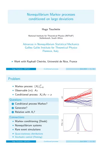
Nonequilibrium Markov processes conditioned on large deviations Chetrite Raphael Laboratoire J.A. Dieudonne Nice FRANCE New Frontiers in Non-equilibrium Physics of Glassy Materials Kyoto, JAPAN August 2015 • Work with Hugo Touchette (Stellenbosch, South Africa) • PRL 2013 and Ann. Henri Poincar´ e 2014 • New paper: arxiv:1506.05291 Chetrite Raphael (CNRS) Conditioned processes August 2015 1 / 18

Heuristic of Large Deviation ”Improbable events permit themselves the luxury of occurring.” C.Chan 1928 • Random variable A T which converges typically toward � a � Large Deviation How improbable for A T to converge towards a which is different from the typical value � a � (rare events) : LDP: P (A T ≈ a) ≍ exp( − TI(a)) • I ( a ): rate function (or fluctuation functional). • Large deviation theory: 1 Prove the LDP and 2 calculate the rate function. Chetrite Raphael (CNRS) Conditioned processes August 2015 2 / 18

Heuristic of Large Deviation ”Improbable events permit themselves the luxury of occurring.” C.Chan 1928 • Random variable A T which converges typically toward � a � Large Deviation How improbable for A T to converge towards a which is different from the typical value � a � (rare events) : LDP: P (A T ≈ a) ≍ exp( − TI(a)) • I ( a ): rate function (or fluctuation functional). • Large deviation theory: 1 Prove the LDP and 2 calculate the rate function. Chetrite Raphael (CNRS) Conditioned processes August 2015 2 / 18

Conditioning Problem Physical • Nonequilibrium process: { X t } T t =0 • Observable: A T [ x ] • Consider trajectories leading to the constraint A T = a • Construct effective Markov process for forget the constraint Mathematical • Markov process: { X t } T t =0 • Conditioned process: X t | A T = a • ”Deconditionning” : T →∞ ∼ X t | A T = a = Y t ���� � �� � Equivalent Markovian process conditioned Exemple Jump Process : the mercantile view of the scientific life Chetrite Raphael (CNRS) Conditioned processes August 2015 3 / 18

Conditioning Problem Physical • Nonequilibrium process: { X t } T t =0 • Observable: A T [ x ] • Consider trajectories leading to the constraint A T = a • Construct effective Markov process for forget the constraint Mathematical • Markov process: { X t } T t =0 • Conditioned process: X t | A T = a • ”Deconditionning” : T →∞ ∼ X t | A T = a = Y t ���� � �� � Equivalent Markovian process conditioned Exemple Jump Process : the mercantile view of the scientific life Chetrite Raphael (CNRS) Conditioned processes August 2015 3 / 18

Historial Work on ”Deconditionning” In Probability : Doob 1957 • { W t | to go outside [0 , L ] via L } ≡ Y t ���� EQN: dYt dt = 1 Yt + dWt dt • Brownian bridge : { W t | W T = 0 } ≡ Y t ���� EQN: dYt dt = − Yt T − t + dWt dt • Quasi-stationary distributions (Deroch-Seneta 1967): X t | not reaching absorbing state ≡ Y t ���� ���� absorbing non-absorbing Chetrite Raphael (CNRS) Conditioned processes August 2015 4 / 18

Historial Work on ”Deconditionning” In Probability : Doob 1957 • { W t | to go outside [0 , L ] via L } ≡ Y t ���� EQN: dYt dt = 1 Yt + dWt dt • Brownian bridge : { W t | W T = 0 } ≡ Y t ���� EQN: dYt dt = − Yt T − t + dWt dt • Quasi-stationary distributions (Deroch-Seneta 1967): X t | not reaching absorbing state ≡ Y t ���� ���� absorbing non-absorbing Chetrite Raphael (CNRS) Conditioned processes August 2015 4 / 18

Historial Work on ”Deconditionning” In Probability : Doob 1957 • { W t | to go outside [0 , L ] via L } ≡ Y t ���� EQN: dYt dt = 1 Yt + dWt dt • Brownian bridge : { W t | W T = 0 } ≡ Y t ���� EQN: dYt dt = − Yt T − t + dWt dt • Quasi-stationary distributions (Deroch-Seneta 1967): X t | not reaching absorbing state ≡ Y t ���� ���� absorbing non-absorbing Chetrite Raphael (CNRS) Conditioned processes August 2015 4 / 18

But First : in Physics with Schr¨ odinger 1931 Chetrite Raphael (CNRS) Conditioned processes August 2015 5 / 18

Chetrite Raphael (CNRS) Conditioned processes August 2015 6 / 18

Chetrite Raphael (CNRS) Conditioned processes August 2015 7 / 18

Chetrite Raphael (CNRS) Conditioned processes August 2015 8 / 18

Chetrite Raphael (CNRS) Conditioned processes August 2015 9 / 18

Chetrite Raphael (CNRS) Conditioned processes August 2015 10 / 18

Diffusion Process • SDE: (with additive noise here for simplicity) dX t = F ( X t ) dt + σ dW t x H t L • One or many particles • Equilibrium or nonequilibrium t • Includes external forces, reservoirs • Generator: ∂ t p ( x , t ) = L † p ( x , t ) ∂ t E x [ f ( X t )] = E x [ Lf ( X t )] , L = F · ∇ + D 2 ∇ 2 , D = σσ T • Path distribution: P [0 , T ] [ x ] Chetrite Raphael (CNRS) Conditioned processes August 2015 11 / 18

Diffusion Process • SDE: (with additive noise here for simplicity) dX t = F ( X t ) dt + σ dW t x H t L • One or many particles • Equilibrium or nonequilibrium t • Includes external forces, reservoirs • Generator: ∂ t p ( x , t ) = L † p ( x , t ) ∂ t E x [ f ( X t )] = E x [ Lf ( X t )] , L = F · ∇ + D 2 ∇ 2 , D = σσ T • Path distribution: P [0 , T ] [ x ] Chetrite Raphael (CNRS) Conditioned processes August 2015 11 / 18

Diffusion Process • SDE: (with additive noise here for simplicity) dX t = F ( X t ) dt + σ dW t x H t L • One or many particles • Equilibrium or nonequilibrium t • Includes external forces, reservoirs • Generator: ∂ t p ( x , t ) = L † p ( x , t ) ∂ t E x [ f ( X t )] = E x [ Lf ( X t )] , L = F · ∇ + D 2 ∇ 2 , D = σσ T • Path distribution: P [0 , T ] [ x ] Chetrite Raphael (CNRS) Conditioned processes August 2015 11 / 18

Observable - random variable • Path x t over [0 , T ] • General observable: x H t L � T � T A T = 1 f ( X t ) dt + 1 g ( X t ) ◦ dX t T T 0 0 t P ( A T = a ) • Large deviation principle (LDP): T = 100 I ( a ) P ( A T = a ) ≈ e − TI ( a ) , T → ∞ T = 50 T = 10 s µ Examples • Occupation time, mean speed, empirical drift • Work, heat, probability current, entropy production • Jump process: current, activity Chetrite Raphael (CNRS) Conditioned processes August 2015 12 / 18

Observable - random variable • Path x t over [0 , T ] • General observable: x H t L � T � T A T = 1 f ( X t ) dt + 1 g ( X t ) ◦ dX t T T 0 0 t P ( A T = a ) • Large deviation principle (LDP): T = 100 I ( a ) P ( A T = a ) ≈ e − TI ( a ) , T → ∞ T = 50 T = 10 s µ Examples • Occupation time, mean speed, empirical drift • Work, heat, probability current, entropy production • Jump process: current, activity Chetrite Raphael (CNRS) Conditioned processes August 2015 12 / 18

Observable - random variable • Path x t over [0 , T ] • General observable: x H t L � T � T A T = 1 f ( X t ) dt + 1 g ( X t ) ◦ dX t T T 0 0 t P ( A T = a ) • Large deviation principle (LDP): T = 100 I ( a ) P ( A T = a ) ≈ e − TI ( a ) , T → ∞ T = 50 T = 10 s µ Examples • Occupation time, mean speed, empirical drift • Work, heat, probability current, entropy production • Jump process: current, activity Chetrite Raphael (CNRS) Conditioned processes August 2015 12 / 18

Conditioned process • Path microcanonical ensemble : a , [0 , T ] [ x ] ≡ P ([ x ] / A T = a ) = P [0 , T ] [ x ] δ ( A T [ x ] − a ) P micro P ( A T = a ) • Intermediate : Path Canonical Ensemble k , [0 , T ] [ x ] ≡ P [0 , T ] [ x ] exp ( kTA T ) P cano E P (exp ( kTA T )) • Motivation in Physics for the Thermodynamics of Trajectories : • Conditioned view to Sheared Fluids (M.Evans). • Dynamical Phase transition for Kinetically constrained models (V.Lecomte, F.Van Wijland,...). • Rare trajectories of Glassy phases (D.Chandler, J.P Garrahan...) Chetrite Raphael (CNRS) Conditioned processes August 2015 13 / 18

Conditioned process • Path microcanonical ensemble : a , [0 , T ] [ x ] ≡ P ([ x ] / A T = a ) = P [0 , T ] [ x ] δ ( A T [ x ] − a ) P micro P ( A T = a ) • Intermediate : Path Canonical Ensemble k , [0 , T ] [ x ] ≡ P [0 , T ] [ x ] exp ( kTA T ) P cano E P (exp ( kTA T )) • Motivation in Physics for the Thermodynamics of Trajectories : • Conditioned view to Sheared Fluids (M.Evans). • Dynamical Phase transition for Kinetically constrained models (V.Lecomte, F.Van Wijland,...). • Rare trajectories of Glassy phases (D.Chandler, J.P Garrahan...) Chetrite Raphael (CNRS) Conditioned processes August 2015 13 / 18

Conditioned process • Path microcanonical ensemble : a , [0 , T ] [ x ] ≡ P ([ x ] / A T = a ) = P [0 , T ] [ x ] δ ( A T [ x ] − a ) P micro P ( A T = a ) • Intermediate : Path Canonical Ensemble k , [0 , T ] [ x ] ≡ P [0 , T ] [ x ] exp ( kTA T ) P cano E P (exp ( kTA T )) • Motivation in Physics for the Thermodynamics of Trajectories : • Conditioned view to Sheared Fluids (M.Evans). • Dynamical Phase transition for Kinetically constrained models (V.Lecomte, F.Van Wijland,...). • Rare trajectories of Glassy phases (D.Chandler, J.P Garrahan...) Chetrite Raphael (CNRS) Conditioned processes August 2015 13 / 18