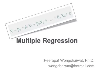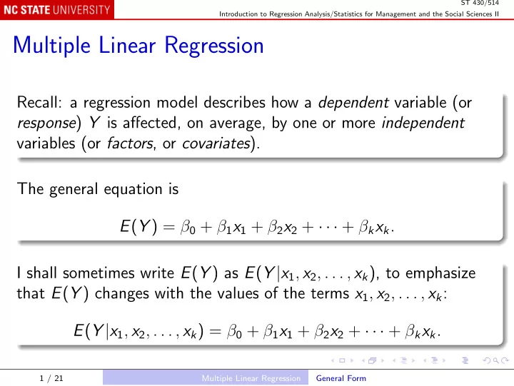
Multiple Linear Regression Recall: a regression model describes how a - - PowerPoint PPT Presentation

ST 430/514 Introduction to Regression Analysis/Statistics for Management and the Social Sciences II

Multiple Linear Regression

Recall: a regression model describes how a dependent variable (or response) Y is affected, on average, by one or more independent variables (or factors, or covariates). The general equation is E(Y ) = β0 + β1x1 + β2x2 + · · · + βkxk. I shall sometimes write E(Y ) as E(Y |x1, x2, . . . , xk), to emphasize that E(Y ) changes with the values of the terms x1, x2, . . . , xk: E(Y |x1, x2, . . . , xk) = β0 + β1x1 + β2x2 + · · · + βkxk.

1 / 21 Multiple Linear Regression General Form

ST 430/514 Introduction to Regression Analysis/Statistics for Management and the Social Sciences II

As always, we can write ǫ = Y − E(Y ),

• r

Y = E(Y ) + ǫ, where the random error ǫ has expected value zero: E(ǫ) = E(ǫ|x1, x2, . . . , xk) = 0. So the general equation can also be written Y = β0 + β1x1 + β2x2 + · · · + βkxk + ǫ.

2 / 21 Multiple Linear Regression General Form

ST 430/514 Introduction to Regression Analysis/Statistics for Management and the Social Sciences II

Each term on the right hand side may be an independent variable, or a function of one or more independent variables. For instance, E(Y ) = β0 + β1x + β2x2 has two terms on the right hand side (not counting the intercept β0), but only one independent variable. We write it in the general form as E(Y ) = β0 + β1x1 + β2x2, with x1 = x and x2 = x2.

3 / 21 Multiple Linear Regression General Form

ST 430/514 Introduction to Regression Analysis/Statistics for Management and the Social Sciences II

Interpreting the parameters: β0 β0 is still called the intercept, but now its interpretation is the expected value of Y when all independent variables are zero: β0 = E(Y |x1 = 0, x2 = 0, . . . , xk = 0). In some cases, these values cannot all be achieved at the same time; in these cases, β0 has only a hypothetical meaning.

4 / 21 Multiple Linear Regression General Form

ST 430/514 Introduction to Regression Analysis/Statistics for Management and the Social Sciences II

Interpreting the parameters: βi, i > 0 For 1 ≤ i ≤ k, βi measures the change in E(Y ) as xi increases by 1 with all the other independent variables held fixed. Again, in some cases it is not possible to change one variable and none of the others, so βi may also have only a hypothetical meaning. You will sometimes find, for instance, some βi < 0 when you expect that Y should increase, not decrease, when xi increases. That is usually because, when xi changes, other variables also change.

5 / 21 Multiple Linear Regression General Form

ST 430/514 Introduction to Regression Analysis/Statistics for Management and the Social Sciences II

Quantitative and Qualitative Variables Some variables are measured quantities (i.e., on an interval or ratio scale), and are called quantitative. Others are the result of classification into categories (i.e. on a nominal or ordinal scale), and are called qualitative. Some terms may be functions of independent variables: distance and distance2, or sine and cosine of (month/12). The simplest case is when all variables are quantitative, and no mathematical functions appear: the first-order model.

6 / 21 Multiple Linear Regression General Form

ST 430/514 Introduction to Regression Analysis/Statistics for Management and the Social Sciences II

Example: Grandfather clocks

Dependence of auction price of antique clocks on their age, and the number of bidders at the auction. Data for 32 clocks. Get the data and plot them:

clocks = read.table("Text/Exercises&Examples/GFCLOCKS.txt", header = TRUE) pairs(clocks[, c("PRICE", "AGE", "NUMBIDS")])

The first-order model is E(PRICE) = β0 + β1 × AGE + β2 × NUMBIDS.

7 / 21 Multiple Linear Regression General Form

ST 430/514 Introduction to Regression Analysis/Statistics for Management and the Social Sciences II

Fitting the model: least squares

As in the case k = 1, the most common way of fitting a multiple regression model is by least squares. That is, find ˆ β0, ˆ β1, . . . , ˆ βk so that ˆ y = ˆ β0 + ˆ β1x1 + . . . ˆ βkxk minimizes SSE =

• (yi − ˆ

yi)2. As noted earlier, other criteria such as |yi − ˆ yi| are sometimes used instead.

8 / 21 Multiple Linear Regression Fitting the model: least squares

ST 430/514 Introduction to Regression Analysis/Statistics for Management and the Social Sciences II

Calculus leads to k + 1 linear equations in the k + 1 estimates ˆ β0, ˆ β1, . . . , ˆ βk. These equations are always consistent; that is, they always have a solution. Usually, they are also non-singular; that is, the solution is unique. If they are singular, we can find a unique solution by either imposing constraints on the parameters or leaving out redundant variables.

9 / 21 Multiple Linear Regression Fitting the model: least squares

ST 430/514 Introduction to Regression Analysis/Statistics for Management and the Social Sciences II

The equations are: n ˆ β0 +

• xi,1 ˆ

β1 + · · · +

• xi,k ˆ

βk =

• yi
• xi,1 ˆ

β0 +

• x2

i,1 ˆ

β1 + · · · +

• xi,1xi,k ˆ

βk =

• xi,1yi

. . .

• xi,k ˆ

β0 +

• xi,1xi,k ˆ

β1 + · · · +

• x2

i,k ˆ

βk =

• xi,kyi

where xi,j is the value in the ith observation of the jth variable, 1 ≤ i ≤ n, 1 ≤ j ≤ k. We usually write these more compactly using matrix notation, and solve them using matrix methods.

10 / 21 Multiple Linear Regression Fitting the model: least squares

ST 430/514 Introduction to Regression Analysis/Statistics for Management and the Social Sciences II

Matrix formulation of least squares Write X for the n × (k + 1) matrix of values of the independent variables (including a column of 1’s for the intercept): X =      1 x1,1 x1,2 . . . x1,k 1 x2,1 x2,2 . . . x2,k . . . . . . . . . ... . . . 1 xn,1 xn,2 . . . xn,k      . Also write y for the n × 1 vector of values of the dependent variable: y =      y1 y2 . . . yn      .

11 / 21 Multiple Linear Regression Fitting the model: least squares

ST 430/514 Introduction to Regression Analysis/Statistics for Management and the Social Sciences II

Finally, write ˆ β for the k × 1 vector of parameter estimates: ˆ β =      ˆ β0 ˆ β1 . . . ˆ βk      Then the equations for the parameter estimates can be written X′Xˆ β = X′y.

12 / 21 Multiple Linear Regression Fitting the model: least squares

ST 430/514 Introduction to Regression Analysis/Statistics for Management and the Social Sciences II

The equations are non-singular when (X′X)−1 exists, and the solution may be written ˆ β = (X′X)−1X′y. However, computing first X′X and then its inverse (X′X)−1 can lead to large numerical errors. Using a transformation of X such as the QR decomposition or the singular value decomposition gives better numerical performance.

13 / 21 Multiple Linear Regression Fitting the model: least squares

ST 430/514 Introduction to Regression Analysis/Statistics for Management and the Social Sciences II

Model Assumptions

No assumptions are needed to find least squares estimates. To use them to make statistical inferences, we need these assumptions: The random errors ǫ1, ǫ2, . . . , ǫn are uncorrelated and have common variance σ2; For small sample validity, the random errors are normally distributed, at least approximately.

14 / 21 Multiple Linear Regression Estimating Error Variance

ST 430/514 Introduction to Regression Analysis/Statistics for Management and the Social Sciences II

As before, we estimate σ2 using SSE =

• (yi − ˆ

yi)2. We can show that E [SSE] = (n − p)σ2, where p = k + 1 is the number of βs in the model, so the unbiased estimator is s2 = SSE dfE = SSE n − p. = SSE n − (k + 1).

15 / 21 Multiple Linear Regression Estimating Error Variance

ST 430/514 Introduction to Regression Analysis/Statistics for Management and the Social Sciences II

Hypothesis Tests

Usually, the first test is an overall test of the model: H0 : β1 = β2 = · · · = βk = 0. Ha : at least one βi = 0. H0 asserts that none of the independent variables affects Y ; if this hypothesis is not rejected, the model is worthless. For instance, its predictions perform no better than ¯ y. The test statistic is usually denoted F, and P-values are found from the F-distribution with k and n − p = n − (k + 1) degrees of freedom.

16 / 21 Multiple Linear Regression Testing the Utility of a Model

ST 430/514 Introduction to Regression Analysis/Statistics for Management and the Social Sciences II

Individual parameters may also be tested: H0 : βi = 0. Ha : βi = 0. The test statistic is t = ˆ βi standard error of ˆ βi It is tested using the t-distribution with n − p degrees of freedom.

17 / 21 Multiple Linear Regression Inferences About Individual Parameters

ST 430/514 Introduction to Regression Analysis/Statistics for Management and the Social Sciences II

Note When you test H0 : βi = 0, you allow the other βs to be non-zero. So with k = 2, you may find that you reject the overall null hypothesis β1 = β2 = 0, but do not reject either β1 = 0 or β2 = 0!

18 / 21 Multiple Linear Regression Inferences About Individual Parameters

ST 430/514 Introduction to Regression Analysis/Statistics for Management and the Social Sciences II

Confidence Intervals A confidence interval for any parameter is constructed in the usual way: ˆ βi ± tα/2,n−(k+1) × standard error. But bear in mind that each such interval has probability α of not covering the true value βi. If you construct many such intervals, there is a greater chance that at least one of them fails to cover its true value.

19 / 21 Multiple Linear Regression Inferences About Individual Parameters

ST 430/514 Introduction to Regression Analysis/Statistics for Management and the Social Sciences II

Example: Grandfather clocks again

Dependence of auction price of antique clocks on their age, and the number of bidders at the auction. Fit the first-order model and summarize it:

clocksLm = lm(PRICE ~ AGE + NUMBIDS, clocks) summary(clocksLm)

20 / 21 Multiple Linear Regression Example

ST 430/514 Introduction to Regression Analysis/Statistics for Management and the Social Sciences II

Output

Call: lm(formula = PRICE ~ AGE + NUMBIDS, data = clocks) Residuals: Min 1Q Median 3Q Max

• 206.49 -117.34

16.66 102.55 213.50 Coefficients: Estimate Std. Error t value Pr(>|t|) (Intercept) -1338.9513 173.8095

• 7.704 1.71e-08 ***

AGE 12.7406 0.9047 14.082 1.69e-14 *** NUMBIDS 85.9530 8.7285 9.847 9.34e-11 ***

• Signif. codes:

0 *** 0.001 ** 0.01 * 0.05 . 0.1 1 Residual standard error: 133.5 on 29 degrees of freedom Multiple R-squared: 0.8923, Adjusted R-squared: 0.8849 F-statistic: 120.2 on 2 and 29 DF, p-value: 9.216e-15

21 / 21 Multiple Linear Regression Example