Markov random fields 2. conditional specifications 3. conditional - PowerPoint PPT Presentation

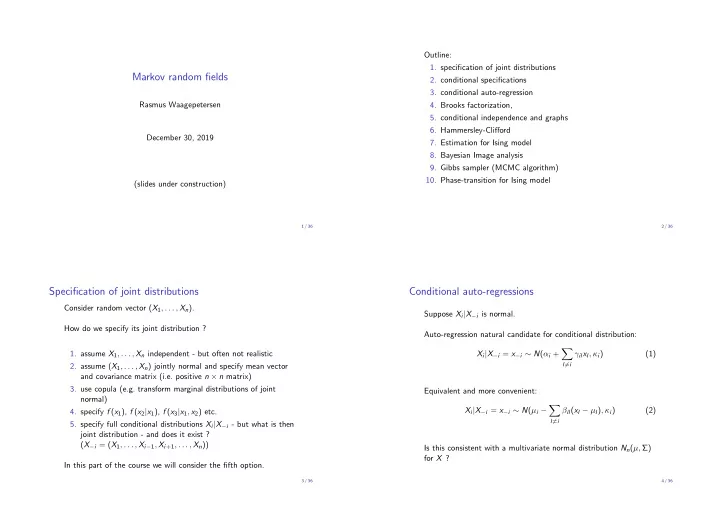
Outline: 1. specification of joint distributions Markov random fields 2. conditional specifications 3. conditional auto-regression Rasmus Waagepetersen 4. Brooks factorization, 5. conditional independence and graphs 6. Hammersley-Clifford December 30, 2019 7. Estimation for Ising model 8. Bayesian Image analysis 9. Gibbs sampler (MCMC algorithm) 10. Phase-transition for Ising model (slides under construction) 1 / 36 2 / 36 Specification of joint distributions Conditional auto-regressions Consider random vector ( X 1 , . . . , X n ). Suppose X i | X − i is normal. How do we specify its joint distribution ? Auto-regression natural candidate for conditional distribution: � 1. assume X 1 , . . . , X n independent - but often not realistic X i | X − i = x − i ∼ N ( α i + γ il x l , κ i ) (1) 2. assume ( X 1 , . . . , X n ) jointly normal and specify mean vector l � = i and covariance matrix (i.e. positive n × n matrix) 3. use copula (e.g. transform marginal distributions of joint Equivalent and more convenient: normal) � X i | X − i = x − i ∼ N ( µ i − β il ( x l − µ l ) , κ i ) (2) 4. specify f ( x 1 ), f ( x 2 | x 1 ), f ( x 3 | x 1 , x 2 ) etc. l � = i 5. specify full conditional distributions X i | X − i - but what is then joint distribution - and does it exist ? ( X − i = ( X 1 , . . . , X i − 1 , X i +1 , . . . , X n )) Is this consistent with a multivariate normal distribution N n ( µ, Σ) for X ? In this part of the course we will consider the fifth option. 3 / 36 4 / 36

Brook’s lemma Application to conditional normal specification Consider two outcomes x and y of X where X has joint density p where p ( y ) > 0. We let y = µ = ( µ 1 , . . . , µ n ). Then � p ( x i | x 1 , . . . , x i − 1 , µ i +1 , . . . , µ n ) � Brooks factorization: log p ( µ i | x 1 , . . . , x i − 1 , µ i +1 , . . . , µ n ) n p ( x ) p ( x i | x 1 , . . . , x i − 1 , y i +1 , . . . , y n ) � p ( y ) = i − 1 i − 1 = − 1 p ( y i | x 1 , . . . , x i − 1 , y i +1 , . . . , y n ) β il ( x l − µ l )) 2 − ( � � β il ( x l − µ l ) 2 ] [( x i − µ i + i =1 2 κ i l =1 l =1 Note n ! ways to factorize ! i − 1 = − 1 [( x i − µ i ) 2 + 2 � β il ( x i − µ i )( x l − µ l )] If conditional densities consistent with joint density, we can choose 2 κ i l =1 fixed y and determine p ( x ) by So p ( x ) ∝ p ( x ) / p ( y ) n n log p ( x ) = log p ( µ ) − 1 β il � � ( x i − µ i )( x l − µ l ) 2 κ i where RHS evaluated using Brook’s factorization. i =1 l =1 with β ii = 1. NB strictly speaking we should write p i ( ·| x − i ) to be able to distinguish different conditional characteristics - but will be lazy. 5 / 36 6 / 36 Conditional distribution of X i for N ( µ, Q − 1 ) p ( x i | x − i ) ∝ exp( − 1 2( x i − µ i ) 2 Q ii − � ( x i − µ i )( x k − µ k ) Q ik ) This is formally equivalent to a multivariate Gaussian density with k � = i mean vector µ and precision matrix Q = Σ − 1 = [ q ij ] ij with For a normal distribution Y ∼ N ( ξ, σ 2 ), q ij = β ij /κ i . p ( y ) ∝ exp( − 1 2 σ 2 y 2 + 1 A well-defined Gaussian density provided Q is symmetric and σ 2 y ξ ) positive definite (whereby Σ = Q − 1 positive definite and symmetric) Comparing the two above equations we get X i | X − i = x − i ∼ N ( µ i − 1 � Q ik ( x k − µ k ) , Q − 1 ii ) Q ii k � = i Thus auto-regressions on slide 4 are in fact general forms of the conditional distributions for a multivariate normal distribution ! 7 / 36 8 / 36

Example: Gaussian random field on 1D lattice Example: Gaussian random field on 2D lattice Consider lattice V = { ( l , k ) | l = 1 , . . . , L , k = 1 , . . . , K } . Now indices i , j ∈ V correspond to points ( i 1 , i 2 ) and ( j 1 , j 2 ) Define i , j ∈ V to be neighbours ⇔ | i 1 − i 2 | + | j 1 − j 2 | = 1 ( i and j horizontal or vertical neighbours). Consider lattice V = { l | l = 1 , . . . , L } . Define µ i = 0, κ i = β ii = 1 and Tempting: define β ii = 1 and β ij = 1 / # N i where # N i is number β ij = β ⇔ | i − j | mod ( L − 2) = 1 of neighbours (2, 3, or 4) of i and κ i = κ > 0. Q obviously symmetric. Q not positive definite if β = − 1 / 2. Problem: resulting Q is positive semi definite: x T Qx = 0 ⇔ x = a 1 n for some a ∈ R . Q positive definite ⇔ | β | < 1 / 2 (exercise in case L = 4 - consider determinant of Q ) We can modify by Q := Q + τ I where τ > 0. Then modified Q is positive definite and we obtain modified conditional distributions κ 1 κ � X i | X − i = x − i ∼ N ( µ i − ( x k − µ k ) , 1 + τ ) κ (1 + τ ) # N i k � = i 9 / 36 10 / 36 Markov random fields Hammersley-Clifford Consider a positive density for X = ( X i ) i ∈ V and a graph G = ( V , E ). Then the following statements are equivalent: Let V denote a finite set of vertices and E a set of edges where an element e in E is of the form { i , j } for i � = j ∈ V . (i.e. an edge is a 1. X is a MRF wrt G . unordered pair of vertices). G = ( V , E ) is a graph. 2. � p ( x ) = φ C ( x C ) i , j ∈ V are neighbours, i ∼ j , if { i , j } ∈ E . C ⊆ V for interaction functions φ C where φ C = 1 unless C is a clique A random vector X = ( X i ) i ∈ V is a Markov random field with wrt. G . We can further introduce the constraint φ C ( x C ) = 1 respect to G if if x l = y l for l ∈ C and some fixed y . Then the interaction p ( x i | x − i ) = p ( x i | x N i ) functions are uniquely determined by the full conditionals. where N i is the set of neighbours of i and for x = ( x l ) l ∈ V and Notation: for ease of notation we often write i for { i } and A ⊆ V , x A = ( x i ) i ∈ A . ( x A , y B ) will denote a vector with entries x i for i ∈ A and y j for j ∈ B , A ∩ B = ∅ (this is a convenient but not rigorous In other words, X i and X j are conditionally independent given notation) X −{ i , j } if i and j are not neighbours. Clique: C ⊆ V is a clique if i ∼ j for all i , j ∈ C . 11 / 36 12 / 36

Proof: 2. ⇒ 1. 1. ⇒ 2. We choose an arbitrary reference outcome y for X . We then define φ ∅ = p ( y ) and, recursively, � C not a clique or x l = y l for some l ∈ C 1 φ C ( x C ) = p ( x C , y − C ) otherwise � B ⊂ C φ B ( x B ) � Let x = ( x A , y − A ) where x l � = y l for all l ∈ A . We show 2. by p ( x i | x − i ) ∝ φ C ( x C ) induction in the cardinality | A | of A . If | A | = 0 then x = y and C ⊆ V : C ∩ i � = ∅ p ( y ) = φ ∅ so 2. holds. Assume now that 2. holds for | A | = k − 1 RHS depends only on x j ∈ N i : if l ∈ C is not a neighbour of i then where k ≤ | V | and consider A with | A | = k . C can not be a clique. Then φ C ( x C ) = 1 so it does not depend on x l . Assume A is a clique. Then by construction, � p ( x A , y − A ) = φ A ( x A ) φ B ( x B ) B ⊂ A and we are done since for C ⊆ V which is not a subset of A we have φ C (( x A , y − A ) C ) = 1 by construction NB: don’t need induction hypothesis in this case. 13 / 36 14 / 36 Brooks vs. Hammersley-Clifford Assume A is not a clique, i.e. there exist l , j ∈ A so that l �∼ j . Given full conditionals we can use either Brooks or H-C to identify Then simultaneous distribution. p ( x A , y − A ) = p ( x l | x A \ l , y − A ) p ( y l | x A \ l , y − A ) p ( x A \ l , y − A , y l ) However, Brooks in principle yields n ! solutions (possible = p ( x l | x A \{ l , j } , y j , y − A ) non-uniqueness) and we need to check that constructed p ( x ) is p ( y l | x A \{ l , j } , y j , y − A ) p ( x A \ l , y − A , y l ) consistent with given full conditionals. = p ( x l , x A \{ l , j } , y j , y − A ) p ( y l , x A \{ l , j } , y j , y − A ) p ( x A \ l , y − A , y l ) For H-C, we can construct the interaction functions using the full conditionals following the proof of 1. ⇒ 2. For given y these � C ⊆ A \ j φ C ( x C ) interaction functions and hence p ( · ) are uniquely determined by � = φ C ( x C ) � C ⊆ A \{ l , j } φ C ( x C ) the full conditionals. Moreover, we can easily check that the C ⊆ A \ l constructed interaction functions are consistent with the full � = φ C ( x C ) conditionals since C ⊆ A p ( x i | x − i ) ∝ p ( x i | x − i ) � p ( y i | x − i ) = φ ( x C ) where second ”=” by 1. and fourth ”=” by induction. Thus 2. C : i ∈ C also holds in this case. Both for Brooks and H-C, we need to check that the identified (unnormalized) simultaneous density indeed has finite integral ! 15 / 36 16 / 36