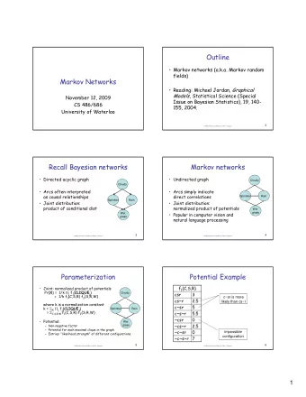
Markov Random Fields and its Applications Huiwen Chang - PowerPoint PPT Presentation

Markov Random Fields and its Applications Huiwen Chang

Introduction • Markov Random Fields(MRF) – A kind of undirected graphical model • To model vision problems: – Low level: image restoration, segmentation, texture analysis… – High level: object recognition and matching(structure from motion, stereo matching)…

Introduction • Markov Random Fields(MRF) – A kind of undirected graphical model • To model vision problems: – Low level: image restoration, segmentation, texture analysis… – High level: object recognition and matching(structure from motion, stereo matching)… Labeling Problem

Graphical Models • Probabilistic graphical models Nodes: random variables Edges: statistical dependencies among random variables – Advantage Compact and efficient way to visualize conditional independence assumptions to represent probability distribution

Conditional Independence

Graphical Model • Bayesian Network – Directed acyclic graph: • Factorization: • Conditional Independence:

Graphical Model • Markov Network (MRF) P(a,b,c,d)= Potential functions over the maximal clique of the graph Potential function ψ (.) > 0

Graphical Model • Markov Network (MRF) P(a,b,c,d)= Hammersley-Clifford theorem says such distributions that are consistent with the set of conditional independence statements & the set of such distributions that can be expressed as a factorization by the maximal cliques of the graph are identical

MAP inference • Posterior probability of the labelling y given observation x is :

Markov Random Field • Posterior probability of the labelling y given observation x is : 1 𝑎(𝑦) 𝜒 𝑑 𝒛 𝐷 ; 𝑦 P( 𝑧 𝑦 = 𝑑 Potential cliques functions where 𝑎(𝑦) = 𝜒 𝑑 𝒛 𝐷 ; 𝑦 is called the partition function . 𝑑 • Since we define potential function is strictly positive, we can express them as exponentials:

MAP inference • Posterior probability of the labelling y given observation x is : • The most possible labeling is to minimize the Energy

Pairwise MRF • Most common energy function for image labeling Unary Pairwise • Which of the energy acted as the prior?

Example MRF model: Image Denoising • How can we retrieve the original image given the noisy one? Original image Y Noisy image X( Input )

MRF formulation • Nodes – For each pixel i, • y i : latent variable (value in original image) • x i : observed variable (value in noisy image) Simple setting : x i , y i  {-1,1} x 1 x 2 y 1 y 2 x i y i x n y n

MRF formulation • Edges – x i ,y i of each pixel i correlated – neighboring pixels, similar value(smoothness) x 1 x 2 y 1 y 2 x i y i x n y n

MRF formulation • Edges – x i ,y i of each pixel i correlated  𝑦 𝑗 , 𝑧 𝑗 = −𝛾𝑦 𝑗 𝑧 𝑗 – neighboring pixels, similar value(smoothness)  ( 𝑧 𝑗 , 𝑧 𝑘 ) = −𝛽𝑧 𝑗 𝑧 𝑘 x 1 x 2 y 1 y 2 x i y i x n y n

MRF formulation Energy function E y; 𝑦 =  ( 𝑧 𝑗 , 𝑧 𝑘 ) +  𝑦 𝑗 , 𝑧 𝑗 𝑗𝑘 𝑗 = −𝛽 𝑧 𝑗 𝑧 𝑘 − 𝛾 𝑦 𝑗 𝑧 𝑗 𝑗𝑘 𝑗 x 1 x 2 y 1 y 2 x i y i x n y n

Optimization Energy function E y; 𝑦 =  ( 𝑧 𝑗 , 𝑧 𝑘 ) +  𝑦 𝑗 , 𝑧 𝑗 𝑗𝑘 𝑗 = −𝛽 𝑧 𝑗 𝑧 𝑘 − 𝛾 𝑦 𝑗 𝑧 𝑗 𝑗𝑘 𝑗 Iterated Conditional Modes (ICM) Initialize 𝑧 𝑗 = 𝑦 𝑗 for all i - Take a 𝑧 𝑗 , fix others, flip 𝑧 𝑗 if −𝑧 𝑗 make energy - lower - Repeat until converge

original image noise image(10%) Restored by ICM(4%)

original image noise image(10%) Restored by ICM(4%) Restored by Graph Cut(<1%)

Optimization • Iterated Conditional Modes(ICM) • Graph Cuts (GC) • Message Passing – Belief Propagation (BP) – Tree Reweighted (not concluded here) • LP-relaxation – Cutting-plane (not concluded here) ……

Graph Cuts • To find labeling f that minimizes the energy E(𝑔; 𝑌) 𝐹 𝑡𝑛𝑝𝑝𝑢ℎ 𝐹 𝑒𝑏𝑢𝑏 𝐸 𝑞 (𝑔 𝑞 ; 𝑌 𝑞 ) neighbors pixels

Graph Cuts • For labeling problem – 2 Labels: Find global minimum • Max-flow/min-cut algorithm • Boykov and Kolmogrov 2001 – the worst case complexity O(mn^2 |C|) – Fast in practice – For multi-labels: Computing the global minimum is NP-hard • Will discuss later

Two-Label Example: Lazy snapping • Goal: Separate foreground from background • 1 st step: Use stroke to select • 2 nd step: Use polygon with vertices to refine

Model the problem 𝐹 1 (𝑦 𝑗 ) : Likelihood Energy 𝐹 2 (𝑦 𝑗 , 𝑦 𝑘 ) : Prior Energy 𝑌 𝑗 : Label of node i. in {0: background , 1: foreground }

Likelihood Energy • Data Term • Use color similarity with known pixel to give an energy for uncertain pixel 𝐺 : Minimum distance to front color – 𝑒 𝑗 𝐶 : Minimum distance to background color – 𝑒 𝑗

Prior Energy • Smoothness Term • Penalty Term for boundaries – Only nonzero if across segmentation boundary – Larger if adjacent pixels have similar colors

Problem • Too slow for “real - time” requirement!

Problem • Too slow for “real - time” requirement!

Pre-segmentation • Graph Cut on segment instead of pixel level • 𝐷 𝑗𝑘 : the mean color difference between the two segments, weighted by the shared boundary length • Speed Comparison

Graph Cuts • 2 Labels: Find global minimum – Max-flow/min-cut algorithm – Fast • Multi-Labels: computing the global minimum is NP-hard – Approximation algorithm(for some forms of energy function: smoothness energy term V which is metric or semi-metric) Identity Symmetry &non-negativity Triangle inequality

Graph Cuts for multi labels • α -expansion(d) – V is metric, within a known factor of global minimum • α  -swap(c) – V is semi-metric, local minimum

Graph Cut for multi labels • α  -swap algorithm – • α -expansion algorithm

Graph Cut for multi labels • α  -swap algorithm – Min cut/ • α -expansion algorithm Max Flow

α  -swap algorithm p r

α -expansion algorithm

Multi-label Examples: Shift Map B C A D User Constraints No accurate segmentation D B C required A

Multi-label Examples: Shift Map B C A D User Constraints D B C A

Multi-label Examples: Shift Map Image completion/In-painting(object removing) User’s mask Input Output

Multi-label Examples: Shift Map Retargeting(content-aware image resizing) Output Input

Multi-label Examples: Shift Map • Label Set: relative mapping coordinate M Labels: shift-map values (t x ,t y ) Nodes: pixels assign a label to (x,y) pixel Input : I(x,y) Output : R(u,v)

Multi-label Examples: Shift Map • Energy function:      ( ) ( ( )) ( ( ), ( )) E M E M p E M p M q d s   , p R p q N Data term : Smoothness term : External Editing Requirement Avoid Stitching Artifacts  0 D • Data term – varies between different application – Inpainting : (x,y) Specific input pixels can be forced not to be included in the output (u,v) image by setting D(x,y )=∞

Smoothness term Output Image Input Image n p’ p’ n q’ p q q’ D iscontinuity in the shift-map For p For q ( ( ), ( )) color E s M p M q gradient

Multi-label Examples: Shift map • Graph Cuts : α -expansion • Why design label as disparity instead of absolute coordinate of input image?

Hierarchical Solution Gaussian pyramid Output on input Shift-Map Shift-Map

Multi-label Examples: Dense Stereo • Label set for each pixel: – disparity 𝑒 ∈ {0, 1, . . 𝐸} Left Camera Image Right Camera Image Dense Stereo Result

Multi-label Examples: Dense Stereo • Data term: for pixel p, label d Left Camera Image Right Camera Image

Multi-label Examples: Dense Stereo • Smoothness term for neighboring pixels p and q – – or,

Design smoothness term V • Choices of V: not Robust Better! = 1 ( 𝛽 − 𝛾 > k) = min (|𝛽 − 𝛾| ,k)

Results Original Image Initial Solution

Results 1 st Expansion Original Image

Results 2 nd Expansion Original Image

Results 3 rd Expansion Original Image

Results Original Image Final expansion

Results • http://vision.middlebury.edu/stereo/eval/

Comments on Graph Cuts • In practice, GraphCut α -expansion algorithm usually outperforms α  -swap method • Limitations of GC algorithm: – Constraint on energy term – Speed

Belief Propagation(BP) • Belief Propagation allows the marginals and maximizer to be computed efficiently on graphical models. • Sum-product BP is a message passing algorithm that calculate the marginal distribution on a graphical model • Max-product BP(or max-sum in log domain), is used to estimate the state configuration with maximum probability. • Exhaustive search O(|state|^N)

Sum-product BP