Markov Networks [KF] Chapter 4 CS 786 University of Waterloo - PDF document

Markov Networks [KF] Chapter 4 CS 786 University of Waterloo Lecture 7: May 24, 2012 Outline • Markov networks – a.k.a. Markov random fields • Conditional random fields 2 CS786 Lecture Slides (c) 2012 P. Poupart 1

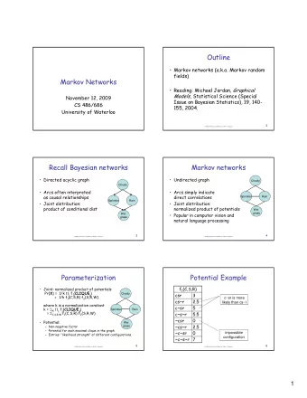
Recall Bayesian networks • Directed acyclic graph Cloudy • Arcs often interpreted as causal relationships Sprinkler Rain • Joint distribution: product of conditional dist Wet grass 3 CS786 Lecture Slides (c) 2012 P. Poupart Markov networks • Undirected graph Cloudy • Arcs simply indicate direct correlations Sprinkler Rain • Joint distribution: normalized product of potentials Wet • Popular in computer vision and grass natural language processing 4 CS786 Lecture Slides (c) 2012 P. Poupart 2

Parameterization • Joint: normalized product of potentials Pr( X ) = 1/k  j f j ( CLIQUE j ) Cloudy = 1/k f 1 (C,S,R) f 2 (S,R,W) where k is a normalization constant k =  X i  j f j ( CLIQUE j ) Sprinkler Rain =  C,S,R,W f 1 (C,S,R) f 2 (S,R,W) • Potential: Wet – Non-negative factor grass – Potential for each maximal clique in the graph – Entries: “likelihood strength” of different configurations. 5 CS786 Lecture Slides (c) 2012 P. Poupart Potential Example f 1 (C,S,R) csr 3 c~sr is more cs~r 2.5 likely than cs~r c~sr 5 c~s~r 5.5 ~csr 0 ~cs~r 2.5 ~c~sr 0 impossible configuration ~c~s~r 7 6 CS786 Lecture Slides (c) 2012 P. Poupart 3

Markov property • Markov property: a variable is independent of all other variables given its immediate neighbours. • Markov blanket: set of direct neighbours B MB(A) = {B,C,D,E} E A C D 7 CS786 Lecture Slides (c) 2012 P. Poupart Conditional Independence • X and Y are independent given Z iff there doesn’t exist any path between X and Y that doesn’t contain any of the variables in Z • Exercise: – A,E? E – A,E|D? A F – A,E|C? G B D – A,E|B,C? C H 8 CS786 Lecture Slides (c) 2012 P. Poupart 4

Interpretation • Markov property has a price: – Numbers are not probabilities • What are potentials? – They are indicative of local correlations • What do the numbers mean? – They are indicative of the likelihood of each configuration – Numbers are usually learnt from data since it is hard to specify them by hand given their lack of a clear interpretation 9 CS786 Lecture Slides (c) 2012 P. Poupart Applications • Natural language processing: – Part of speech tagging • Computer vision – Image segmentation • Any other application where there is no clear causal relationship 10 CS786 Lecture Slides (c) 2012 P. Poupart 5

Image Segmentation Segmentation of the Alps Kervrann, Heitz (1995) A Markov Random Field model-based Approach to Unsupervised Texture Segmentation Using Local and Global Spatial Statistics, IEEE Transactions on Image Processing, vol 4, no 6, p 856-862 11 CS786 Lecture Slides (c) 2012 P. Poupart Image Segmentation • Variables – Pixel features (e.g. intensities): X ij – Pixel labels: Y ij • Correlations: – Neighbouring pixel labels are correlated – Label and features of a pixel are correlated • Segmentation: – argmax Y Pr( Y | X )? 12 CS786 Lecture Slides (c) 2012 P. Poupart 6

Inference • Markov nets: factored representation – Use variable elimination • P( X | E = e )? – Restrict all factors that contain E to e – Sumout all variables that are not X or in E – Normalize the answer 13 CS786 Lecture Slides (c) 2012 P. Poupart Parameter Learning • Maximum likelihood –  * = argmax  P(data|  ) • Complete data – Convex optimization, but no closed form solution – Iterative techniques such as gradient descent • Incomplete data – Non-convex optimization – EM algorithm 14 CS786 Lecture Slides (c) 2012 P. Poupart 7

Maximum likelihood • Let  be the set of parameters and x i be the i th instance in the dataset • Optimization problem: –  * = argmax  P(data|  ) = argmax   i Pr( x i |  ) = argmax   i  j f( X [j]= x i [j])  X  j f( X [j]= x i [j]) where X [j] is the clique of variables that potential j depends on and x [j] is a variable assignment for that clique 15 CS786 Lecture Slides (c) 2012 P. Poupart Maximum likelihood • Let  x = f( X = x ) • Optimization continued: –  * = argmax   i  j  X i [j]  X  j  X i [j] = argmax  log  i  j  X i [j]  X  j  X i [j] = argmax   i  j log  X i [j] – log  X  j  X i [j] • This is a non-concave optimization problem 16 CS786 Lecture Slides (c) 2012 P. Poupart 8

Maximum likelihood • Substitute  = log  and the problem becomes concave : –  * = argmax   i  j  X i [j] – log  X e  j  X i [j] • Possible algorithms: – Gradient ascent – Conjugate gradient 17 CS786 Lecture Slides (c) 2012 P. Poupart Feature-based Markov Networks • Generalization of Markov networks – May not have a corresponding graph – Use features and weights instead of potentials – Use exponential representation • Pr( X = x ) = 1/k e  j  j  j ( x[j] ) where x[j] is a variable assignment for a subset of variables specific to  j • Feature  j : Boolean function that maps partial variable assignments to 0 or 1 • Weight  j : real number 18 CS786 Lecture Slides (c) 2012 P. Poupart 9

Feature-based Markov Networks • Potential-based Markov networks can always be converted to feature-based Markov networks Pr( x ) = 1/k  j f j ( CLIQUE j = x [j]) = 1/k e  j, clique j  j, clique j  j, clique j ( x [j]) •  j, clique j = log f j ( CLIQUE j = x [j]) •  j, clique j ( x [j])=1 if clique j = x [j], 0 otherwise 19 CS786 Lecture Slides (c) 2012 P. Poupart Example weights features f 1 (C,S,R) 1 if CSR = csr  1,csr = log 3  1,csr (CSR) = csr 3 0 otherwise cs~r 2.5 1 if CSR = *s~r  1,*s~r = log 2.5  1,*s~r (CSR) = 0 otherwise c~sr 5 1 if CSR = c~sr  1,c~sr = log 5  c~sr (CSR) = c~s~r 5.5 0 otherwise  1,c~s~r = log 5.5  1,c~s~r (CSR) = 1 if CSR = c~s~r ~csr 0 0 otherwise ~cs~r 2.5  1,~c*r = log 0  1,~c*r (CSR) = 1 if CSR = ~c*r ~c~sr 0 0 otherwise  1,~c~s~r = log 7  ~c~s~r (CSR) = 1 if CSR = ~c~s~r ~c~s~r 7 0 otherwise 20 CS786 Lecture Slides (c) 2012 P. Poupart 10

Features • Features – Any Boolean function – Provide tremendous flexibility • Example: text categorization – Simplest features: presence/absence of a word in a document – More complex features • Presence/absence of specific expressions • Presence/absence of two words within a certain window • Presence/absence of any combination of words • Presence/absence of a figure of style • Presence/absence of any linguistic feature 21 CS786 Lecture Slides (c) 2012 P. Poupart Conditional Random Fields • CRF: special Markov network that represents a conditional distribution • Pr( X | E ) = 1/k( E ) e  j  j  j ( X,E ) – NB: k( E ) is a normalization function (it is not a constant since it depends on E – see Slide 5) • Useful in classification: Pr(class|input) • Advantage: no need to model distribution over inputs 22 CS786 Lecture Slides (c) 2012 P. Poupart 11

Conditional Random Fields • Joint distribution: – Pr( X,E ) = 1/k e  j  j  j ( X,E ) • Conditional distribution – Pr( X | E ) = e  j  j  j ( X,E ) /  X e  j  j  j ( X,E ) • Partition features in two sets: –  j1 ( X,E ): depend on at least one var in X –  j2 ( E ): depend only on evidence E 23 CS786 Lecture Slides (c) 2012 P. Poupart Conditional Random Fields • Simplified conditional distribution: – Pr(X|E) = e  j1  j1  j1 ( X,E ) +  j2  j2  j2 ( E )  X e  j1  j1  j1 ( X,E ) +  j2  j2  j2 ( E ) = e  j1  j1  j1 ( X,E ) e  j2  j2  j2 ( E )  X e  j1  j1  j1 ( X,E ) e  j2  j2  j2 ( E ) = 1/k( E ) e  j1  j1  j1 ( X,E ) • Evidence features can be ignored! 24 CS786 Lecture Slides (c) 2012 P. Poupart 12

Parameter Learning • Parameter learning is simplified since we don’t need to model a distribution over the evidence • Objective: maximum conditional likelihood –  * = argmax  P(X=x|  ,E=e) – Convex optimization, but no closed form – Use iterative technique (e.g., gradient descent) 25 CS786 Lecture Slides (c) 2012 P. Poupart Sequence Labeling • Common task in – Entity recognition – Part of speech tagging – Robot localisation – Image segmentation • L* = argmax L Pr( L | O )? = argmax L 1 ,…,L n Pr(L 1 ,…,L n |O 1 ,…,O n )? 26 CS786 Lecture Slides (c) 2012 P. Poupart 13

Hidden Markov Model S 1 S 2 S 3 S 4 O 1 O 2 O 3 O 4 • Assumption: observations are independent given the hidden state 27 CS786 Lecture Slides (c) 2012 P. Poupart Conditional Random Fields • Since the distribution over observations is not modeled, there is no independence assumption among observations S 1 S 2 S 3 S 4 O 1 O 2 O 3 O 4 • Can also model long-range dependencies without significant computational cost 28 CS786 Lecture Slides (c) 2012 P. Poupart 14