Markov Chains and Coupling In this class we will consider the - PDF document

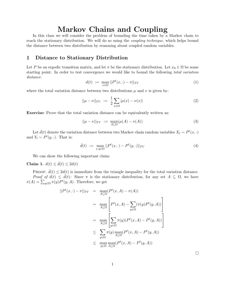
Markov Chains and Coupling In this class we will consider the problem of bounding the time taken by a Markov chain to reach the stationary distribution. We will do so using the coupling technique , which helps bound the distance between two distribution by reasoning about coupled random variables. 1 Distance to Stationary Distribution Let P be an ergodic transition matrix, and let π be the stationary distribution. Let x 0 ∈ Ω be some starting point. In order to test convergence we would like to bound the following total variation distance : x ∈ Ω || P t ( x, · ) − π || TV d ( t ) := max (1) where the total variation distance between two distributions µ and ν is given by: := 1 � || µ − ν || TV | µ ( x ) − ν ( x ) | (2) 2 x ∈ Ω Exercise: Prove that the total variation distance can be equivalently written as: || µ − ν || TV := max A ⊆ Ω ( µ ( A ) − ν ( A )) (3) Let ¯ d ( t ) denote the variation distance between two Markov chain random variables X t ∼ P t ( x, · ) and Y t ∼ P t ( y, · ). That is: ¯ x,y ∈ Ω || P t ( x, · ) − P t ( y, · ) || TV d ( t ) := max (4) We can show the following important claim: Claim 1. d ( t ) ≤ ¯ d ( t ) ≤ 2 d ( t ) Proof: ¯ d ( t ) ≤ 2 d ( t ) is immediate from the triangle inequality for the total variation distance. Proof of d ( t ) ≤ ¯ d ( t ) : Since π is the stationary distribution, for any set A ⊆ Ω, we have y ∈ Ω π ( y ) P t ( y, A ). Therefore, we get π ( A ) = � || P t ( x, · ) − π || TV A ⊆ Ω ( P t ( x, A ) − π ( A )) = max   �  P t ( x, A ) − ( π ( y ) P t ( y, A )) = max  A ⊆ Ω y ∈ Ω   � π ( y )( P t ( x, A ) − P t ( y, A )) = max  A ⊆ Ω y ∈ Ω � A ⊆ Ω ( P t ( x, A ) − P t ( y, A )) ≤ π ( y ) max y ∈ Ω A ⊆ Ω ( P t ( x, A ) − P t ( y, A )) ≤ max y ∈ Ω max 1

The above claim is important since it allows us to quantify the variation distance to the sta- tionary distribution ( d ( t )) using the distance between two Markov chains ( ¯ d ( t )) from the same transition matrix (within a factor of 2). Moreover, it allows us to do so without knowing what the stationary distribution. We will see how to bound ¯ d ( t ) in the rest of the class using coupling techniques. 2 Coupling Coupling is a powerful technique that will help us bound the convergence rates of a Markov chain. Definition 1. Let X and Y be random variables with probability distributions µ and ν on Ω . A distribution ω on Ω × Ω is a coupling if � ∀ x ∈ Ω , w ( x, y ) = µ ( x ) y ∈ Omega � ∀ x ∈ Ω , w ( x, y ) = ν ( y ) x ∈ Omega 2.1 Coupling Lemma Lemma 1. Consider a pair of distributions µ and ν over Ω . (a) For any coupling w of µ and ν , let ( X, Y ) w , || µ − ν || TV ≤ P ( X � = Y ) (b) There always exists a coupling w s.t., || µ − ν || TV = P ( X � = Y ) Proof of (a): For any valid coupling w , ∀ z, w ( z, z ) ≤ min( µ ( z ) , ν ( z )) (5) Therefore, � P ( X � = Y ) = 1 − P ( X = Y ) = 1 − w ( z, z ) z � � ≥ µ ( z ) − min( µ ( z ) , ν ( z )) z z � ≥ ( µ ( z ) − ν ( z )) z : µ ( z ) >ν ( z ) = || µ − ν || TV Proof of (b): We are now going to construct a coupling w s.t. P ( X � = Y ) = || µ − ν || TV . 2

First we fix the diagonal entries: ∀ z, w ( z, z ) = min( µ ( z ) , ν ( z ) This ensures that P ( X � = Y ) indeed equals the total variation distance between the two distribu- tions. We set the off diagonal entries as follow: w ( y, z ) = ( µ ( y ) − w ( y, y ))( ν ( z ) − w ( z, z )) 1 − � x w ( x, x ) We leave it as an exercise to verify that w is indeed a coupling. 3 Coupling and Markov Chains The key insight from the coupling lemma is that the total variation distance between two distribu- tions µ and ν is bounded above by P ( X � = Y ) for any two random variables that are coupled with respect to µ and ν . This turns out to be very useful in the context of Markov chains. First, we know from Claim 1 that the variation distance to the stationary distribution at time t is bounded (within a factor of 2) by the variation distance between any two Markov chains with the same transition matrix at time t . Moreover, by choosing an appropriately couple pair of Markov chains, we can bound || P t ( x, · ) − P t ( y, · ) || TV by the probability P ( X t � = Y t ). Using this coupling argument, we will next prove that an ergodic Markov chain always converges to a unique stationary distribution, and then show a bound on the time taken to convergence (also known as mixing time ) for the problem of randomly sampling graph colorings. 4 Ergodicity Theorem Theorem 1. If P is irreducible and aperiodic, then there is a unique stationary distribution π such that t →∞ P t ( x, · ) = π ∀ x, lim Proof: Consider two copies of the Markov chain X t and Y t , both following P . We create a coupling distribution as follows: • If X t � = Y t , then choose X t +1 and Y t +1 independently according to P . • If X t = Y t , then choose X t +1 ∼ P , and set Y t +1 = X t +1 . From the coupling lemma we know that ∀ t, || X t − Y t || TV ≤ P ( X t � = Y t ) Due to ergodicity, there exist t ⋆ such that ∀ x, y , P t ⋆ ( x, y ) > 0. Therefore, there is some ǫ > 0, such that for all initial states X 0 , Y 0 , P ( X t ⋆ � = Y t ⋆ | X 0 , Y 0 ) ≤ 1 − ǫ (6) Similarly, due to the Markovian property, we can say P ( X 2 t ⋆ � = Y 2 t ⋆ | X t ⋆ � = Y t ⋆ ) ≤ 1 − ǫ (7) 3

Also, due to the coupling, X 2 t ⋆ = Y 2 t ⋆ implies X t ⋆ = Y t ⋆ . Therefore, P ( X 2 t ⋆ � = Y 2 t ⋆ | X 0 , Y 0 ) P ( X t ⋆ � = Y t ⋆ ∧ X 2 t ⋆ � = Y 2 t ⋆ | X 0 , Y 0 ) = P ( X 2 t ⋆ � = Y 2 t ⋆ | X t ⋆ � = Y t ⋆ ) P ( X t ⋆ � = Y t ⋆ | X 0 , Y 0 ) = (1 − ǫ ) 2 ≤ Hence for any integer k > 0, we have P ( X kt ⋆ � = Y kt ⋆ | X 0 , Y 0 ) ≤ (1 − ǫ ) k (8) As k → ∞ , P ( X kt ⋆ � = Y kt ⋆ | X 0 , Y 0 ) → 0. Since X t and Y t are coupled such that once they are the same at time t , they are the same for all t ′ > t , we have t →∞ P ( X t � = Y t | X 0 , Y 0 ) → 0 lim From the coupling lemma, we have || P t ( x, · ) − P t ( y, · ) || TV ≤ P ( X t � = Y t ) → 0 , when t → 0 To verify that, σ = lim t →∞ P t ( x, · ) is the required stationary distribution, note that � � t →∞ P t ( z, x ) P ( x, y ) ∀ z σ ( x ) P ( x, y ) = lim x x t →∞ P t +1 ( z, y ) = σ ( y ) = lim This shows that σP = σ . Also, σ is unique since || lim t →∞ P t ( x, · ) − lim t →∞ P t ( y, · ) || TV → 0. 5 Mixing Time Recall the definition of d ( t ). || P t ( x, · ) − π || TV d ( t ) = max d x ( t ) = max x x We can show that d ( t ) is non-decreasing in t . Claim 2. d x ( t ) is non-decreasing in t . Proof: Let X 0 be some x ∈ Ω, and let Y 0 have the stationary distribution. Fix t . By the coupling lemma, there is a coupling and random variables X t ∼ P t ( x, · ) and Y t ∼ π such that d x ( t ) = || P t ( x, · ) − π || TV = P ( X t � = Y t ) Using this coupling, we define a coupling of the distributions of X t +1 , Y t +1 as follows: • If X t = Y t , set X t +1 = Y t +1 . • Else, let X t → X t +1 and Y t → Y t +1 independently. Then we have, d x ( t + 1) = || P t +1 ( x, · ) − π || TV ≤ P ( X t +1 � = Y t +1 ) ≤ P ( X t � = Y t ) = d x ( t ) The first inequality holds due to the coupling lemma, and the second inequality holds by construc- tion of the coupling. Since d ( t ) never decreases, we can define the mixing time τ ( ǫ ) of a Markov chain as: τ ( ǫ ) = min t { d ( t ) ≤ ǫ } (9) 4