Markov chain algorithms for bounded Heng Guo (University of - PowerPoint PPT Presentation
Markov chain algorithms for bounded Heng Guo (University of Edinburgh) (Shanghai Jiao Tong University) LFCS lab lunch, Mar 10th, 2020 degree k -Sat Joint with Weiming Feng, Yitong Yin (Nanjing University) and Chihao Zhang Satisfiability One of
Markov chain algorithms for bounded Heng Guo (University of Edinburgh) (Shanghai Jiao Tong University) LFCS lab lunch, Mar 10th, 2020 degree k -Sat Joint with Weiming Feng, Yitong Yin (Nanjing University) and Chihao Zhang
Satisfiability One of the most important problem in computer science Output: Is it satisfiable? Input: A formula in conjunctive normal form, like ( x 1 ∨ x 3 ∨ x 5 ) ∧ ( x 2 ∨ x 3 ) ∧ ( x 3 ∨ x 4 ) ∧ ( x 1 ∨ x 5 ∨ x 6 ∨ x 7 ) . . . The first NP -complete problem Cook (1971) — Levin (1973)
Sampling solutions Sometimes we are not satisfied with finding one solution. We want to gen- The ability of sampling solutions enables us to • approximately count the number of solutions; • estimate the marginal probability of individual variables; • estimate other quantities of interest … And sometimes generating random instances satisfying given constraints can be useful too. local lemma conditions). erate a uniformly at random solution. Sampling can be NP -hard even if finding a solution is easy (e.g. under Lovász
A natural (but not working) approach Standard sampling approach: Glauber dynamics / Gibbs sampling
A natural (but not working) approach Standard sampling approach: Glauber dynamics / Gibbs sampling Choose a random variable, sample its value conditioned on all others. T/F ?? T ! T ?? T F T T T T T T x 1 x 1 x 2 x 2 x 3 x 4 x 5 x 6 x 7 x 8 C 1 C 2 C 3 C 4 ( ¬ x 1 ∨ x 2 ∨ x 5 ) ∧ ( ¬ x 2 ∨ ¬ x 6 ∨ x 7 ) ∧ ( x 1 ∨ ¬ x 3 ∨ ¬ x 7 ) ∧ ( ¬ x 4 ∨ x 6 ∨ x 8 )
A natural (but not working) approach Standard sampling approach: Glauber dynamics / Gibbs sampling Choose a random variable, sample its value conditioned on all others. T/F ?? T ! T ?? T F T T T T T T x 1 x 1 x 2 x 2 x 3 x 4 x 5 x 6 x 7 x 8 C 1 C 2 C 3 C 4 ( ¬ x 1 ∨ x 2 ∨ x 5 ) ∧ ( ¬ x 2 ∨ ¬ x 6 ∨ x 7 ) ∧ ( x 1 ∨ ¬ x 3 ∨ ¬ x 7 ) ∧ ( ¬ x 4 ∨ x 6 ∨ x 8 )
A natural (but not working) approach Standard sampling approach: Glauber dynamics / Gibbs sampling Choose a random variable, sample its value conditioned on all others. T/F ?? T ! T ?? T F T T T T T T x 1 x 1 x 2 x 2 x 3 x 4 x 5 x 6 x 7 x 8 C 1 C 2 C 3 C 4 ( ¬ x 1 ∨ x 2 ∨ x 5 ) ∧ ( ¬ x 2 ∨ ¬ x 6 ∨ x 7 ) ∧ ( x 1 ∨ ¬ x 3 ∨ ¬ x 7 ) ∧ ( ¬ x 4 ∨ x 6 ∨ x 8 )
A natural (but not working) approach Standard sampling approach: Glauber dynamics / Gibbs sampling Choose a random variable, sample its value conditioned on all others. T/F ?? T ! T ?? T F T T T T T T x 1 x 1 x 2 x 2 x 3 x 4 x 5 x 6 x 7 x 8 C 1 C 2 C 3 C 4 ( ¬ x 1 ∨ x 2 ∨ x 5 ) ∧ ( ¬ x 2 ∨ ¬ x 6 ∨ x 7 ) ∧ ( x 1 ∨ ¬ x 3 ∨ ¬ x 7 ) ∧ ( ¬ x 4 ∨ x 6 ∨ x 8 )
A natural (but not working) approach Standard sampling approach: Glauber dynamics / Gibbs sampling Choose a random variable, sample its value conditioned on all others. T/F ?? T ! T ?? T F T T T T T T x 1 x 1 x 2 x 2 x 3 x 4 x 5 x 6 x 7 x 8 C 1 C 2 C 3 C 4 ( ¬ x 1 ∨ x 2 ∨ x 5 ) ∧ ( ¬ x 2 ∨ ¬ x 6 ∨ x 7 ) ∧ ( x 1 ∨ ¬ x 3 ∨ ¬ x 7 ) ∧ ( ¬ x 4 ∨ x 6 ∨ x 8 )
A natural (but not working) approach Standard sampling approach: Glauber dynamics / Gibbs sampling Choose a random variable, sample its value conditioned on all others. T/F ?? T ! T ?? T F T T T T T T x 1 x 1 x 2 x 2 x 3 x 4 x 5 x 6 x 7 x 8 C 1 C 2 C 3 C 4 ( ¬ x 1 ∨ x 2 ∨ x 5 ) ∧ ( ¬ x 2 ∨ ¬ x 6 ∨ x 7 ) ∧ ( x 1 ∨ ¬ x 3 ∨ ¬ x 7 ) ∧ ( ¬ x 4 ∨ x 6 ∨ x 8 )
A natural (but not working) approach Standard sampling approach: Glauber dynamics / Gibbs sampling Choose a random variable, sample its value conditioned on all others. T/F ?? T ! T ?? T F T T T T T T x 1 x 1 x 2 x 2 x 3 x 4 x 5 x 6 x 7 x 8 C 1 C 2 C 3 C 4 ( ¬ x 1 ∨ x 2 ∨ x 5 ) ∧ ( ¬ x 2 ∨ ¬ x 6 ∨ x 7 ) ∧ ( x 1 ∨ ¬ x 3 ∨ ¬ x 7 ) ∧ ( ¬ x 4 ∨ x 6 ∨ x 8 )
Three scenarios for Markov chains Fast mixing Slow mixing Not mixing! We are here!
Three scenarios for Markov chains Fast mixing Slow mixing Not mixing! We are here!
(using . . clauses), the solution space is not connected via single variable updates. . Disconnectivity for k -Sat Suppose we have k variables, and each clause contains all k variables. Φ = C 1 ∧ C 2 ∧ · · · ∧ C m Each C i forbids one assignment on k variables. For example, C i = x 1 ∨ x 2 ∨ · · · ∨ x k forbids the all False assignment. Thus, if we forbade all assignments of Hamming weight i for some 1 ⩽ i ⩽ k − 1 ( k ) i For example, to remove Hamming weight k − 1 assignments, we only need clauses C 1 = ¬ x 1 ∨ x 2 ∨ . . . x k C 2 = x 1 ∨ ¬ x 2 ∨ . . . x k C k = x 1 ∨ x 2 ∨ . . . ¬ x k In this example, the all False assignment is disconnected from the rest.
(using . . clauses), the solution space is not connected via single variable updates. . Disconnectivity for k -Sat Suppose we have k variables, and each clause contains all k variables. Φ = C 1 ∧ C 2 ∧ · · · ∧ C m Each C i forbids one assignment on k variables. For example, C i = x 1 ∨ x 2 ∨ · · · ∨ x k forbids the all False assignment. Thus, if we forbade all assignments of Hamming weight i for some 1 ⩽ i ⩽ k − 1 ( k ) i For example, to remove Hamming weight k − 1 assignments, we only need clauses C 1 = ¬ x 1 ∨ x 2 ∨ . . . x k C 2 = x 1 ∨ ¬ x 2 ∨ . . . x k C k = x 1 ∨ x 2 ∨ . . . ¬ x k In this example, the all False assignment is disconnected from the rest.
Our solution — projection Projecting from a high dimension to a lower dimension may improve con- nectivity. We will run Glauber dynamics on the projected distribution over a suitably “marked” variables. The general problem is NP -hard, so we will focus on bounded degree cases.
Bounded degree k -Sat
Lovász local lemma Theorem (Loász local lemma) Let E 1 , . . . , E m be a set of “bad” events, such that Pr [ E i ] ⩽ p for all i . More- over, each E i is independent from all but at most ∆ events. If ep∆ ⩽ 1 , then [ m ] ∧ Pr E i > 0. i = 1 In the setuing of k -Sat, each clause C i defines a bad event E i , which is the forbidden assignment of C i , and p = 2 − k . If every variable appears in at most d clauses, then ∆ ⩽ kd . ep∆ ⩽ 1 ⇔ e2 − k kd ⩽ 1 ⇔ k ⩾ log d + log k + C
Lovász local lemma Theorem (Loász local lemma) Let E 1 , . . . , E m be a set of “bad” events, such that Pr [ E i ] ⩽ p for all i . More- over, each E i is independent from all but at most ∆ events. If ep∆ ⩽ 1 , then [ m ] ∧ Pr E i > 0. i = 1 In the setuing of k -Sat, each clause C i defines a bad event E i , which is the forbidden assignment of C i , and p = 2 − k . If every variable appears in at most d clauses, then ∆ ⩽ kd . ep∆ ⩽ 1 ⇔ e2 − k kd ⩽ 1 ⇔ k ⩾ log d + log k + C
Moser-Tardos algorithm Theorem (Moser and Tardos, 2011) polynomial time. The algorithm is extremely simple: assign variables u.a.r., then keep resam- ple variables in violating clauses. Unfortunately, sampling is substantially harder. Theorem (Bezáková, Galanis, Goldberg, G. and Štefankovič, 2016) there is no negation in the formula (monotone case). We consider k -CNF formula with variable degree at most d . If k ⩾ log d + log k + C , then we can always find a satisfying assignment in If k ⩽ 2 log d + C , then sampling satisfying assignments is NP -hard, even if
Moser-Tardos algorithm Theorem (Moser and Tardos, 2011) polynomial time. The algorithm is extremely simple: assign variables u.a.r., then keep resam- ple variables in violating clauses. Unfortunately, sampling is substantially harder. Theorem (Bezáková, Galanis, Goldberg, G. and Štefankovič, 2016) there is no negation in the formula (monotone case). We consider k -CNF formula with variable degree at most d . If k ⩾ log d + log k + C , then we can always find a satisfying assignment in If k ⩽ 2 log d + C , then sampling satisfying assignments is NP -hard, even if
Open problem: Is there an efficient algorithm to sample satisfying assignments of k - Sat given k ≳ 2 log d + C ?
Results formula). Theorem (Our result) We give a Markov chain based algorithm in Hermon, Sly and Zhang (2016) Glauber dynamics mixes in O ( n log n ) time if k ⩾ 2 log d + C and there is no negation (monotone G., Jerrum and Liu (2016) “Partial rejection sampling” terminates in O ( n ) time if k ⩾ 2 log d + C and there is no small intersection. Moitra (2016) An “exotic” deterministic algorithm in n O ( k 2 d 2 ) time if k ⩾ 60 ( log d + log k ) + 300 . � O ( n 1 + δ k 3 d 2 ) time if k ⩾ 20 ( log d + log k ) + log δ − 1 where δ ⩽ 1/60 is an arbitrary constant.
Results formula). Theorem (Our result) We give a Markov chain based algorithm in Hermon, Sly and Zhang (2016) Glauber dynamics mixes in O ( n log n ) time if k ⩾ 2 log d + C and there is no negation (monotone G., Jerrum and Liu (2016) “Partial rejection sampling” terminates in O ( n ) time if k ⩾ 2 log d + C and there is no small intersection. Moitra (2016) An “exotic” deterministic algorithm in n O ( k 2 d 2 ) time if k ⩾ 60 ( log d + log k ) + 300 . � O ( n 1 + δ k 3 d 2 ) time if k ⩾ 20 ( log d + log k ) + log δ − 1 where δ ⩽ 1/60 is an arbitrary constant.
Our algorithm
Recommend
More recommend
Explore More Topics
Stay informed with curated content and fresh updates.
