Introduction 1 SAT planning Introduction 2 SAT planning vs. - PowerPoint PPT Presentation

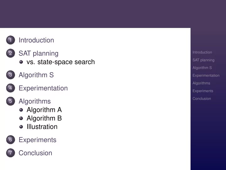
Introduction 1 SAT planning Introduction 2 SAT planning vs. state-space search Algorithm S Algorithm S 3 Experimentation Algorithms Experimentation 4 Experiments Conclusion 5 Algorithms Algorithm A Algorithm B Illustration Experiments 6 Conclusion 7

Introduction SAT planning Evaluation Strategies for Planning as Algorithm S Satisfiability Experimentation Algorithms Experiments Conclusion Jussi Rintanen Albert-Ludwigs-Universität Freiburg, Germany August 26, ECAI’04

Introduction We consider evaluation strategies for satisfiability Introduction planning: find a (not necessarily shortest) plan. SAT planning Trade-off: quality vs. cost to produce. Algorithm S Experimentation Application domain: any approach to planning in Algorithms which basic step is finding a plan of a given length, Experiments like planning as satisfiability, by CSP , by MILP , Conclusion Graphplan, ... Significance: speed-ups of 0, 1, 2, 3, 4, ... orders of magnitude in comparison to the standard sequential evaluation strategy (as used in Graphplan, BLACKBOX, ...)

Strengths of satisfiability planning (SATP) Satisfiability planning (Kautz & Selman, 1992/96) is an Introduction SAT planning efficient approach for solving inherently difficult planning vs. state-space search problems: Algorithm S optimal solutions to otherwise easy problems Experimentation Algorithms (Most of the standard planning benchmarks are Experiments solvable non-optimally by simple poly-time Conclusion algorithms!!!) hard problems in the phase transition region [Rintanen, KR’04] combinatorially difficult planning problems

SATP vs. heuristic state-space planning Heuristic state-space search [Bonet & Geffner 2000] has Introduction been considered stronger than SATP on many SAT planning non-optimal planning problems, but vs. state-space search Algorithm S apples vs. oranges: SATP planners give optimality Experimentation guarantees but planners like HSP do not, and Algorithms nobody has used SATP planners for non-optimal Experiments planning. Conclusion Open question How efficient SATP actually is when optimality is not required?

SATP for non-optimal planning Goal Non-optimal planning: relax all optimality Introduction requirements, any plan will do! SAT planning vs. state-space search Consequence SATP becomes extremely good on Algorithm S standard big-and-easy benchmarks. Experimentation Algorithms Disclaimer Problems that are very easy and very big Experiments likely remain to be solved by more Conclusion specialized planning techniques: After all, SAT solvers are general-purpose problem solvers and cannot be as efficient as more specialized techniques on all types of problems.

The standard sequential evaluation algorithm Formula φ j represents the question Is there a plan of length j ? Introduction SAT planning Algorithm S PROCEDURE AlgorithmS() Experimentation Algorithms i := 0 ; Experiments REPEAT Conclusion test satisfiability of φ i ; IF φ i is satisfiable THEN terminate; i := i + 1 ; UNTIL 1=0; Problem This algorithm proves that the plan has optimal length!!!

Experimentation Introduction How do runtime profiles of different benchmarks look SAT planning like? Algorithm S benchmarks from planning competitions 1998, 2000, 1 Experimentation 2002 Algorithms samples from the set of all instances [Rintanen 2 Experiments KR’04] Conclusion Tests were run with Siege SAT solver version 4 (by Lawrence Ryan of University of Washington and Synopsys). This is one of the best SAT solvers for planning problems.

Examples Evaluation times: logistics39-0 700 Introduction SAT planning 600 Algorithm S Experimentation 500 Algorithms time in secs 400 Experiments Conclusion 300 200 100 0 0 2 4 6 8 10 12 14 16 18 20 time points

Examples Evaluation times: gripper10 500 Introduction 450 SAT planning Algorithm S 400 Experimentation 350 Algorithms time in secs 300 Experiments 250 Conclusion 200 150 100 50 0 0 10 20 30 40 50 60 time points

Examples Evaluation times: satell20 700 Introduction SAT planning 600 Algorithm S Experimentation 500 Algorithms time in secs 400 Experiments Conclusion 300 200 100 0 0 5 10 15 20 25 time points

Examples Evaluation times: schedule51 400 Introduction SAT planning 350 Algorithm S 300 Experimentation Algorithms time in secs 250 Experiments 200 Conclusion 150 100 50 0 0 5 10 15 20 25 30 time points

Examples Evaluation times: blocks22 40 Introduction SAT planning 35 Algorithm S 30 Experimentation Algorithms time in secs 25 Experiments 20 Conclusion 15 10 5 0 0 10 20 30 40 50 60 70 80 90 100 time points

Examples Evaluation times: depot15 200 Introduction 180 SAT planning Algorithm S 160 Experimentation 140 Algorithms time in secs 120 Experiments 100 Conclusion 80 60 40 20 0 0 5 10 15 20 time points

Difficult problems with 20 state variables Introduction Sampled from the space of all problems instances SAT planning with 20 state variables, 40 or 42 STRIPS operators Algorithm S each having 3 precondition literals and 2 effect Experimentation literals. Algorithms Experiments This is in the phase transition region [Rintanen, Conclusion KR’04]. We show here some of the most difficult instances. Easier instances are solved (by satisfiability planners) in milliseconds.

Examples Evaluation times: random1024 14 Introduction SAT planning 12 Algorithm S Experimentation 10 Algorithms time in secs 8 Experiments Conclusion 6 4 2 0 0 5 10 15 20 25 30 35 40 45 50 time points

Examples Evaluation times: random6076 18 Introduction 16 SAT planning Algorithm S 14 Experimentation 12 Algorithms time in secs Experiments 10 Conclusion 8 6 4 2 0 0 10 20 30 40 50 60 time points

Examples Evaluation times: random2315 25 Introduction SAT planning Algorithm S 20 Experimentation Algorithms time in secs 15 Experiments Conclusion 10 5 0 0 5 10 15 20 25 30 35 40 45 time points

Examples Evaluation times: random8597 25 Introduction SAT planning Algorithm S 20 Experimentation Algorithms time in secs 15 Experiments Conclusion 10 5 0 0 10 20 30 40 50 60 time points

The important insight 10.0 Introduction SAT planning cost of evaluation Characteristic shape: Algorithm S 5.0 Most of the difficulty is Experimentation 3.0 in the last unsatisfiable 1.0 1.0 Algorithms 0.5 0.1 0.1 0.2 formulae. Experiments 1 2 3 4 5 6 7 8 9 plan length Conclusion Devise evaluation 1 2 3 1 2 3 1 (1) (1) run by process strategies that get to evaluate the easier satisfiable formulae early!!

Algorithm A Introduction SAT planning Algorithm S n processes: evaluate n plan lengths simultaneously Experimentation (starting from lengths 0 to n − 1 ) Algorithms Algorithm A When a process finishes one length, in continues Algorithm B Illustration with the first unallocated one. Experiments Special case n = 1 is Algorithm S. Conclusion

Algorithm B Evaluate all plan lengths simultaneously at different Introduction rates. SAT planning Algorithm S If rate of length n is r , evaluate length n +1 at rate γr . Experimentation γ is a constant 0 < γ < 1 . Algorithms The CPU times allocated to the formulae form a Algorithm A Algorithm B geometric sequence Illustration Experiments tγ 0 , tγ 1 , tγ 2 , . . . Conclusion with a finite sum t 1 − γ .

Properties of Algorithm B Introduction The first unfinished formula gets 1 − γ of the CPU. SAT planning With γ = 0 . 9 this is 1 10 , with γ = 0 . 5 it is 1 2 . Algorithm S Experimentation Speed-up is between 1 − γ and ∞ . Algorithms runtime with Algorithm S Algorithm A Speed-up = Algorithm B runtime with Algorithm B Illustration Experiments Conclusion Worst-case slow-down only a constant factor! Speed-up can be arbitrarily high!!

Algorithm B with γ = 0 . 9 Finding a plan for blocks22 with Algorithm B 45 Introduction 40 SAT planning Algorithm S 35 Experimentation 30 Algorithms time in secs Algorithm A 25 Algorithm B Illustration 20 Experiments Conclusion 15 10 5 0 40 45 50 55 60 65 70 75 80 85 90 time points

Algorithm B with γ = 0 . 9 Finding a plan for blocks22 with Algorithm B 45 Introduction 40 SAT planning Algorithm S 35 Experimentation 30 Algorithms time in secs Algorithm A 25 Algorithm B Illustration 20 Experiments Conclusion 15 10 5 0 40 45 50 55 60 65 70 75 80 85 90 time points

Algorithm B with γ = 0 . 9 Finding a plan for blocks22 with Algorithm B 45 Introduction 40 SAT planning Algorithm S 35 Experimentation 30 Algorithms time in secs Algorithm A 25 Algorithm B Illustration 20 Experiments Conclusion 15 10 5 0 40 45 50 55 60 65 70 75 80 85 90 time points

Algorithm B with γ = 0 . 9 Finding a plan for blocks22 with Algorithm B 45 Introduction 40 SAT planning Algorithm S 35 Experimentation 30 Algorithms time in secs Algorithm A 25 Algorithm B Illustration 20 Experiments Conclusion 15 10 5 0 40 45 50 55 60 65 70 75 80 85 90 time points