Linear Regression Yijun Zhao Northeastern University Fall 2016 - PowerPoint PPT Presentation
Linear Regression Yijun Zhao Northeastern University Fall 2016 Yijun Zhao Linear Regression Regression Examples Any Attributes Continuous Value = x y { age , major , gender , race } GPA { income , credit score , profession }
Linear Regression Yijun Zhao Northeastern University Fall 2016 Yijun Zhao Linear Regression
Regression Examples Any Attributes Continuous Value = ⇒ x y { age , major , gender , race } ⇒ GPA { income , credit score , profession } ⇒ loan { college , major , GPA } ⇒ future income . . . Yijun Zhao Linear Regression
Regression Examples Data often has/can be converted into matrix form: Age Gender Race Major GPA 20 0 A Art 3.85 22 0 C Engineer 3.90 25 1 A Engineer 3.50 24 0 AA Art 3.60 19 1 H Art 3.70 18 1 C Engineer 3.00 30 0 AA Engineer 3.80 25 0 C Engineer 3.95 28 1 A Art 4.00 26 0 C Engineer 3.20 Yijun Zhao Linear Regression
Formal Problem Setup Given N observations { ( x 1 , y 1 ) , ( x 2 , y 2 ) , . . . , ( x N , y N ) } a regression problem tries to uncover the function y i = f ( x i ) ∀ i = 1 , 2 . . . . , n such that for a new input value x ∗ , we can accurately predict the corresponding value y ∗ = f ( x ∗ ). Yijun Zhao Linear Regression
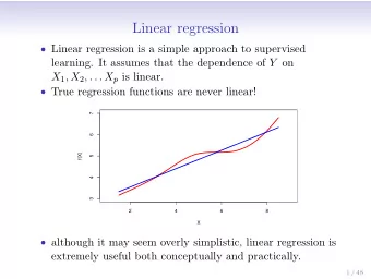
Linear Regression Assume the function f is a linear combination of components in x Formally, let x = (1 , x 1 , x 2 , . . . , x d ) T , we have y = ω 0 + ω 1 x 1 + ω 2 x 2 + · · · + ω d x d = w T x where w = ( ω 0 , ω 1 , ω 2 , . . . , ω d ) T w is the parameter to estimate ! Prediction: y ∗ = w T x ∗ Yijun Zhao Linear Regression
Visual Illustration Figure: 1D and 2D linear regression Yijun Zhao Linear Regression
Error Measure Mean Squared Error (MSE): N E ( w ) = 1 � ( w T x n − y n ) 2 N n =1 = 1 N � Xw − y � 2 where — x 1 T — y 1 — x 2 T — y 2 X = y = . . . . . . — x NT — y N Yijun Zhao Linear Regression
Minimizing Error Measure E ( w ) = 1 N � Xw − y � 2 ▽ E ( w ) = 2 N X T ( Xw − y ) = 0 X T Xw = X T y w = X † y where X † = ( X T X ) − 1 X T is the ’pseudo-inverse’ of X Yijun Zhao Linear Regression
LR Algorithm Summary Ordinary Least Squares (OLS) Algorithm Construct matrix X and the vector y from the dataset { ( x 1 , y 1 ) , x 2 , y 2 ) , . . . , ( x N , y N ) } (each x includes x 0 = 1) as follows: — x T 1 — y 1 — x T 2 — y 2 X = y = . . . . . . — x T N — y N Compute X † = ( X T X ) − 1 X T Return w = X † y Yijun Zhao Linear Regression
Gradient Descent Why? Minimize our target function ( E ( w )) by moving down in the steepest direction Yijun Zhao Linear Regression
Gradient Descent Gradient Descent Algorithm Initialize the w (0) for time t = 0 for t = 0 , 1 , 2 , . . . do Compute the gradient g t = ▽ E ( w ( t )) Set the direction to move, v t = − g t Update w ( t + 1) = w ( t ) + η v t Iterate until it is time to stop Return the final weights w Yijun Zhao Linear Regression
Gradient Descent How η affects the algorithm? Use 0.1 (practical observation) Use variable size: η t = η � ▽ E � Yijun Zhao Linear Regression
OLS or Gradient Descent? Yijun Zhao Linear Regression
Computational Complexity OLS Gradient Descent ¡ OLS is expensive when D is large! Yijun Zhao Linear Regression
Linear Regression What is the Probabilistic Interpretation? Yijun Zhao Linear Regression
Normal Distribution Right Skewed Left Skewed Random Yijun Zhao Linear Regression
Normal Distribution mean = median = mode symmetry about the center 2 σ 2 ( x − µ ) 2 1 2 π e − x ∼ N ( µ, σ 2 ) = 1 ⇒ f ( x ) = √ σ Yijun Zhao Linear Regression
Central Limit Theorem All things bell shaped! Random occurrences over a large population tend to wash out the asymmetry and uniformness of individual events. A more ’natural’ distribution ensues. The name for it is the Normal distribution (the bell curve). Formal definition: If ( y 1 , . . . , y n ) are i.i.d. and 0 < σ 2 y < ∞ , then when n is large the distribution of ¯ y is well approximated by a σ 2 normal distribution N ( µ y , n ). y Yijun Zhao Linear Regression
Central Limit Theorem Example: Yijun Zhao Linear Regression
LR: Probabilistic Interpretation Yijun Zhao Linear Regression
LR: Probabilistic Interpretation 2 πσ e − 1 2 σ 2 ( w T x i − y i ) 2 1 prob ( y i | x i ) = √ Yijun Zhao Linear Regression
LR: Probabilistic Interpretation Likelihood of the entire dataset: e − 1 2 σ 2 ( w T x i − y i ) 2 � � � L ∝ i − 1 ( w T x i − y i ) 2 � 2 σ 2 = e i ( w T x i − y i ) 2 Maximize L ⇐ ⇒ Minimize � i Yijun Zhao Linear Regression
Non-linear Transformation Linear is limited: Linear models become powerful when we consider non-linear feature transformations: X i = (1 , x i , x 2 ⇒ y i = ω 0 + ω 1 x i + ω 2 x 2 i ) = i Yijun Zhao Linear Regression
Overfitting Yijun Zhao Linear Regression
Overfitting How do we know we overfitted? E in : Error from the training data E out : Error from the test data Example: Yijun Zhao Linear Regression
Overfitting How to avoid overfitting? Use more data Evaluate on a parameter tuning set Regularization Yijun Zhao Linear Regression
Regularization Attempts to impose ”Occam’s razor” principle Add a penalty term for model complexity Most commonly used : L 2 regularization (ridge regression) minimizes: E ( w ) = � Xw − y � 2 + λ � w � 2 where λ ≥ 0 and � w � 2 = w T w L 1 regularization (LASSO) minimizes: E ( w ) = � Xw − y � 2 + λ | w | 1 D � where λ ≥ 0 and | w | 1 = | ω i | i =1 Yijun Zhao Linear Regression
Regularization L 2: closed form solution w = ( X T X + λ I ) − 1 X T y L 1: No closed form solution. Use quadratic programming: minimize � Xw − y � 2 � w � 1 ≤ s s . t . Yijun Zhao Linear Regression
L 2 Regularization Example Yijun Zhao Linear Regression
Model Selection Which model? A central problem in supervised learning Simple model: ”underfit” the data Constant function Linear model applied to quadratic data Complex model: ”overfit” the data High degree polynomials Model with hidden logics that fits the data to completion Yijun Zhao Linear Regression
Bias-Variance Trade-off � � N 1 ( w T x n − y n ) 2 y = w T x n � Consider E let ˆ N n =1 y − y n ) 2 can be decomposed into (reading): E (ˆ var { noise } + bias 2 + var { y i } var { noise } : can’t be reduced bias 2 + var { y i } is what counts for prediction High bias 2 : model mismatch, often due to ”underfitting” High var { y i } : training set and test set mismatch, often due to ”overfitting” Yijun Zhao Linear Regression
Bias-Variance Trade-off Often: low bias ⇒ high variance low variance ⇒ high bias Trade-off: Yijun Zhao Linear Regression
How to choose λ ? But we still need to pick λ . Use the test set data ? NO! Set aside another evaluation set Small evaluation set ⇒ inaccurate estimated error Large evaluation set ⇒ small training set CrossValidation Yijun Zhao Linear Regression
Cross Validation (CV) Divide data into K folds Alternatively train on all except k th folds, and test on k th fold Yijun Zhao Linear Regression
Cross Validation (CV) How to choose K? Common choice of K = 5 , 10, or N (LOOCV) Measure on average performance Cost of computation: K folds × choices of λ Yijun Zhao Linear Regression
Learning Curve A learning curve plots the performance of the algorithm as a function of the size of training data Yijun Zhao Linear Regression
Learning Curve Yijun Zhao Linear Regression
Recommend
More recommend
Explore More Topics
Stay informed with curated content and fresh updates.
