CSSE463: Image Recognition Day 5 Demo code posted Lab 2 due - PowerPoint PPT Presentation

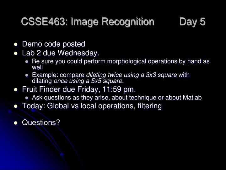
CSSE463: Image Recognition Day 5  Demo code posted  Lab 2 due Wednesday.  Be sure you could perform morphological operations by hand as well  Example: compare dilating twice using a 3x3 square with dilating once using a 5x5 square .  Fruit Finder due Friday, 11:59 pm.  Ask questions as they arise, about technique or about Matlab  Today: Global vs local operations, filtering  Questions?

Global vs. local operators  Global operators  Use information from the entire image  p~ = f(p, p img)  Local operators  Transform each pixel based on its value or its neighbors’ values only  p~ = f(p, p p N ) Q1

Enhancement: gray-level mapping  Maps each pixel value to another value  Could use a lookup table, e.g., [(0,0), (1, 3), (2, 5), …]  Could use a function  Identity mapping, y=x is straight line  Function values above y=x are boosted, those below are suppressed.  Gamma function, y = x^(1/g) (assuming x in range [0,1]) is a common a control in monitors/TVs.  g=2 shown to left  Effect? Q2

Gamma mappings, y = x^(1/g) Original Dark (g = 0.5) Light (g = 2) Very light (g = 4)

Histogram Equalization  Creates a mapping that flattens the histogram.  Uses full range [0, 255]  Good: “automatically” enhances contrast where needed.  Approx same level of pixels of each gray level  Unpredictable results.  Maintains the histogram’s shape, but changes the density of the histogram  Good example of a global operation  Next: pros and cons

HistEq on Sunset

HistEq on Matt

But where’s the color?  Can we use gray-level mapping on color images?  Discuss how Q3

Local operators  The most common local operators are filters .  Today: for smoothing  Tomorrow: for edge detection

Image smoothing  Gaussian distributions are often used to model noise in the image  g = g r + N(0, )  g = sensed gray value  g r = “expected” real grayvalue  N(0, ) is a Gaussian (aka, N ormal, or bell curve) with mean = 0, std. dev = .  Lots of Gaussian distributions in this course…  Answer: average it out! 3 methods  Box filter  Gaussian filter  Median filter  Filter

Box filters  Simplest.  Improves homogeneous regions.  Unweighted average of the pixels in a small neighborhood.  For 5x5 neighborhood, 2 2 1 J ( r , c ) I ( r i , c j ) 25 i 2 j 2 See why this is a “local operation?” I = orig image, J=filtered image

Gaussian filters  Nicest theoretical properties.  Average weighted by distance from center pixel. Weight of pixel (i,j): 2 d 1 2 2 W ( i , j ) e 2  Then use weight in box filter formula  In practice, we use a discrete approximation to W(i,j)

Median filters  Averaging filters have two  Step edge demo problems.  smoothGaussDemo  They blur edges.  Salt demo  They don’t do well with “salt -and- pepper” noise:  smoothSaltDemo  Faulty CCD elements  Dust on lens  Median filter: Replace each pixel with the median of the pixels in its neighborhood  More expensive  Harder to do with hardware  But can be made somewhat efficient  (Sonka, p 129) Q4,5  Hybrid: sigma filtering

Discrete filters 1 / 9 1 / 9 1 / 9  Discrete 3x3 box filter: 1 / 9 1 / 9 1 / 9  To get the output at a 1 / 9 1 / 9 1 / 9 single point, take cross- correlation (basically a dot-product) of filter and image at that point  To filter the whole image, shift the filter over each pixel in the original image