Linear Regression Let us assume that the target variable and the - PDF document
School of Computer Science Learning generalized linear models and tabular CPT of structured full BN Probabilistic Graphical Models (10- Probabilistic Graphical Models (10 -708) 708) Lecture 9, Oct 15, 2007 Receptor A Receptor A X 1 X 1 X
School of Computer Science Learning generalized linear models and tabular CPT of structured full BN Probabilistic Graphical Models (10- Probabilistic Graphical Models (10 -708) 708) Lecture 9, Oct 15, 2007 Receptor A Receptor A X 1 X 1 X 1 Receptor B Receptor B X 2 X 2 X 2 Eric Xing Eric Xing Kinase C Kinase C X 3 X 3 X 3 Kinase D Kinase D X 4 X 4 X 4 Kinase E Kinase E X 5 X 5 X 5 TF F TF F X 6 X 6 X 6 Reading: J-Chap. 7,8. Gene G Gene G X 7 X 7 X 7 X 8 X 8 X 8 Gene H Gene H 1 Linear Regression � Let us assume that the target variable and the inputs are related by the equation: = θ T + ε y x i i i where ε is an error term of unmodeled effects or random noise � Now assume that ε follows a Gaussian N (0, σ ), then we have: 1 ⎛ 2 ⎞ − θ T y ( ) x θ = ⎜ − ⎟ p y x i i ( | ; ) exp ⎜ ⎟ 2 2 i i 2 σ π σ ⎝ ⎠ Eric Xing 2 1
Logistic Regression (sigmoid classifier) � The condition distribution: a Bernoulli 1 1 = µ y − µ − y p y x x x ( | ) ( ) ( ( )) where µ is a logistic function 1 µ = x ( ) 1 − θ T + x e � We can used the brute-force gradient method as in LR � But we can also apply generic laws by observing the p ( y | x ) is an exponential family function, more specifically, a generalized linear model Eric Xing 3 Exponential family � For a numeric random variable X { } X n η = η T − η p x h x T x A ( | ) ( ) exp ( ) ( ) N 1 { } = η h x T T x ( ) exp ( ) η Z ( ) is an exponential family distribution with natural (canonical) parameter η � Function T ( x ) is a sufficient statistic . � Function A( η ) = log Z( η ) is the log normalizer. � Examples: Bernoulli, multinomial, Gaussian, Poisson, gamma,... Eric Xing 4 2
Multivariate Gaussian Distribution � For a continuous vector random variable X ∈ R k : 1 1 ⎧ ⎫ − 1 µ Σ = − − µ T Σ − µ p x ⎨ x x ⎬ ( , ) exp ( ) ( ) ( ) 1 2 2 2 2 π k Σ / ⎩ ⎭ / Moment parameter 1 { ( ) } = − Σ − 1 + µ Σ − 1 − µ Σ − 1 µ − Σ 1 xx T T x 1 T exp tr log ( ) 2 2 2 2 π k / � Exponential family representation Natural parameter [ ( ) ] [ ] ( ) − 1 − 1 − 1 − 1 η = Σ µ − 1 Σ = η η η = Σ µ η = − 1 Σ ; vec , vec , and 1 2 1 2 2 2 [ ( ) ] = T T x x xx ( ) ; vec ( ) η = µ Σ − 1 µ + Σ = − η η η − − 2 η 1 T 1 T 1 A ( ) log tr ( ) log 2 2 2 1 1 2 2 ( ) 2 2 − k = π / h x ( ) Note: a k -dimensional Gaussian is a ( d + d 2 )-parameter distribution with a ( d + d 2 )- � element vector of sufficient statistics (but because of symmetry and positivity, parameters are constrained and have lower degree of freedom) Eric Xing 5 Multinomial distribution x x π ~ multi ( | ), � For a binary vector random variable ⎧ ⎫ ∑ 1 2 K π = π x π x π x = k π p x ⎨ x ⎬ ( ) L exp ln 1 2 K k ⎩ ⎭ k ⎧ ⎫ − 1 ⎛ − − 1 ⎞ ⎛ − − 1 ⎞ K K K ∑ ∑ ∑ 1 1 = k π + ⎜ K ⎟ ⎜ π ⎟ ⎨ x x ⎬ exp ln ln k k ⎩ ⎝ ⎠ ⎝ ⎠ ⎭ = 1 = 1 = 1 k k k ⎧ ⎫ 1 ⎛ π ⎞ ⎛ − 1 ⎞ K − K − ∑ ∑ ⎜ ⎟ 1 = k + ⎜ π ⎟ x k exp ⎨ ln ln ⎬ ⎜ ⎟ 1 1 − ∑ K − π k ⎝ ⎠ ⎝ ⎠ ⎩ ⎭ = 1 = 1 k = 1 k k k � Exponential family representation ⎡ π ⎤ ⎛ ⎞ η = 0 ⎜ ⎟ ln k ; ⎢ ⎥ π ⎣ ⎝ ⎠ ⎦ K [ ] = T x x ( ) ⎛ − 1 ⎞ ⎛ ⎞ K − K ∑ ∑ 1 η = − ⎜ π ⎟ = ⎜ η ⎟ A e ( ) ln ln k k ⎝ ⎠ ⎝ ⎠ = 1 = 1 k k 1 = h x ( ) Eric Xing 6 3
Why exponential family? � Moment generating property 1 dA d d = η = η Z Z log ( ) ( ) η η η η d d Z d ( ) 1 d { } ∫ = η T h x T x dx ( ) exp ( ) η η Z d ( ) { } η T h x T x ( ) exp ( ) ∫ = T x dx ( ) η Z ( ) [ ] = E T x ( ) { } { } 2 η η 1 d A h x T T x h x T T x d ( ) exp ( ) ( ) exp ( ) ∫ 2 ∫ = − η T x dx T x dx Z ( ) ( ) ( ) 2 η η η η η d Z Z Z d ( ) ( ) ( ) [ ] [ ] 2 = − 2 E T x E T x ( ) ( ) [ ] = Var T x ( ) Eric Xing 7 Moment estimation � We can easily compute moments of any exponential family distribution by taking the derivatives of the log normalizer A ( η ). � The q th derivative gives the q th centered moment. η dA ( ) = mean η d 2 η d A ( ) = variance 2 η d L � When the sufficient statistic is a stacked vector, partial derivatives need to be considered. Eric Xing 8 4
Moment vs canonical parameters � The moment parameter µ can be derived from the natural (canonical) parameter η dA ( ) [ ] def = = µ 8 8 E T x A ( ) η d � A ( h ) is convex since 4 4 2 η d A ( ) [ ] η 0 = > Var T x ( ) η ∗ 2 η d -2 -2 -1 -1 0 0 1 1 2 2 � Hence we can invert the relationship and infer the canonical parameter from the moment parameter (1-to-1): def η = ψ µ ( ) A distribution in the exponential family can be parameterized not only by η − the � canonical parameterization, but also by µ − the moment parameterization. Eric Xing 9 MLE for Exponential Family � For iid data, the log-likelihood is { } ∏ l η = η T − η D h x T x A ( ; ) log ( ) exp ( ) ( ) n n n ⎛ ⎞ ∑ ∑ = + ⎜ η T ⎟ − η h x T x NA log ( ) ( ) ( ) n n ⎝ ⎠ n n � Take derivatives and set to zero: ∂ ∂ η l A ∑ ( ) 0 = − = T x N ( ) n ∂ η ∂ η n 1 ∂ η A ( ) ∑ = T x ( ) n ∂ η N ⇒ n 1 ) ∑ µ = T x ( ) MLE n N n � This amounts to moment matching . ) ) η = ψ µ � We can infer the canonical parameters using ( ) MLE MLE Eric Xing 10 5
Sufficiency � For p ( x | θ ), T ( x ) is sufficient for θ if there is no information in X regarding θ yeyond that in T ( x ). We can throw away X for the purpose pf inference w.r.t. θ . � θ θ = θ p T x x p T x X T ( x ) ( | ( ), ) ( | ( )) � Bayesian view θ = θ p x T x p x T x Frequentist view � X T ( x ) ( | ( ), ) ( | ( )) The Neyman factorization theorem � θ X T ( x ) T ( x ) is sufficient for θ if � θ = ψ θ ψ p x T x T x x T x ( , ( ), ) ( ( ), ) ( , ( )) 1 2 ⇒ θ = θ p x g T x h x T x ( | ) ( ( ), ) ( , ( )) Eric Xing 11 Examples � Gaussian: [ ] ( ) − 1 − 1 η = Σ µ − 1 Σ ; vec 2 [ ] ( ) 1 1 = T T x x xx ∑ ∑ ( ) ; vec ⇒ µ = = T x x ( ) 1 MLE n n N N η = µ Σ − 1 µ + Σ A 1 T 1 ( ) log n n 2 2 ( ) 2 2 − k = π / h x ( ) � Multinomial: ⎡ π ⎤ ⎛ ⎞ 0 η = ⎜ ⎟ ln k ; ⎢ ⎥ π ⎣ ⎝ ⎠ ⎦ K 1 [ ] ∑ = ⇒ µ = T x x x ( ) MLE n N ⎛ − − 1 ⎞ ⎛ ⎞ K K n ∑ ∑ η = − ⎜ 1 π ⎟ = ⎜ η ⎟ A e ( ) ln ln k k ⎝ ⎠ ⎝ ⎠ = 1 = 1 k k 1 = h x ( ) � Poisson: η = λ log = T x x 1 ( ) ∑ ⇒ µ = x η = λ = η A e ( ) MLE n N n 1 = h x ( ) x ! Eric Xing 12 6
Generalized Linear Models (GLIMs) � The graphical model X n Linear regression � Discriminative linear classification � Commonality: � Y n model E p ( Y )= µ = f ( θ T X ) N What is p ()? the cond. dist. of Y. � What is f ()? the response function. � � GLIM The observed input x is assumed to enter into the model via a linear � T x ξ = θ combination of its elements The conditional mean µ is represented as a function f ( ξ ) of ξ , where f is � known as the response function The observed output y is assumed to be characterized by an � exponential family distribution with conditional mean µ . Eric Xing 13 GLIM, cont. θ ψ f µ η ξ x { } η = η − η T p y h y x y A ( | ) ( ) exp ( ) ( ) { } ( ) ⇒ η = 1 η T − η p y h y x y A ( | ) ( ) exp ( ) ( ) φ The choice of exp family is constrained by the nature of the data Y � y is a continuous vector � multivariate Gaussian Example: � y is a class label � Bernoulli or multinomial The choice of the response function � Following some mild constrains, e.g., [0,1]. Positivity … � f − 1 = ψ ( ⋅ ) Canonical response function: � In this case θ T x directly corresponds to canonical parameter η . � Eric Xing 14 7
Recommend
More recommend
Explore More Topics
Stay informed with curated content and fresh updates.
