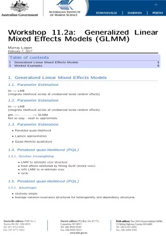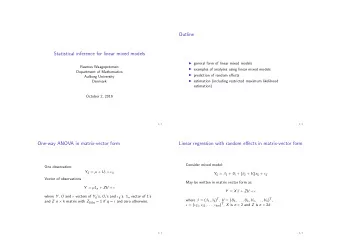
Generalized linear mixed effects models Consider stochastic vector Y - PowerPoint PPT Presentation

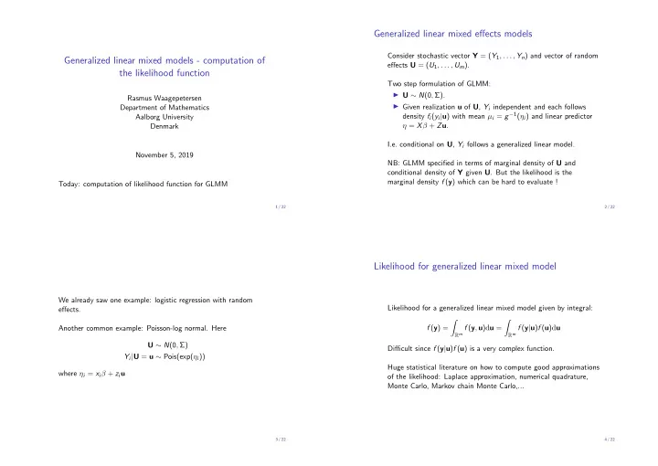
Generalized linear mixed effects models Consider stochastic vector Y = ( Y 1 , . . . , Y n ) and vector of random Generalized linear mixed models - computation of effects U = ( U 1 , . . . , U m ). the likelihood function Two step formulation of GLMM: ◮ U ∼ N (0 , Σ). Rasmus Waagepetersen ◮ Given realization u of U , Y i independent and each follows Department of Mathematics density f i ( y i | u ) with mean µ i = g − 1 ( η i ) and linear predictor Aalborg University η = X β + Z u . Denmark I.e. conditional on U , Y i follows a generalized linear model. November 5, 2019 NB: GLMM specified in terms of marginal density of U and conditional density of Y given U . But the likelihood is the marginal density f ( y ) which can be hard to evaluate ! Today: computation of likelihood function for GLMM 1 / 22 2 / 22 Likelihood for generalized linear mixed model We already saw one example: logistic regression with random Likelihood for a generalized linear mixed model given by integral: effects. � � Another common example: Poisson-log normal. Here f ( y ) = R m f ( y , u ) d u = R m f ( y | u ) f ( u ) d u U ∼ N (0 , Σ) Difficult since f ( y | u ) f ( u ) is a very complex function. Y i | U = u ∼ Pois(exp( η i )) Huge statistical literature on how to compute good approximations where η i = x i β + z i u of the likelihood: Laplace approximation, numerical quadrature, Monte Carlo, Markov chain Monte Carlo,... 3 / 22 4 / 22

Example: logistic regression with random intercepts Hierarchical model with independent random effects U j ∼ N (0 , τ 2 ) , j = 1 , . . . , m Suppose U = ( U 1 , . . . , U m ) with the the U i independent. Y j | U j = u j ∼ binomial( n j , p j ) log( p j / (1 − p j )) = η j = β + U j Moreover Y = ( Y ij ) ij , i = 1 , . . . , m and j = 1 , . . . , n i where the p j = exp( η j ) / (1 + exp( η j )) conditional distribution of the Y = ( Y ij ) j only depends on U i . Then we can factorize likelihood as m Conditional density: � � f ( y ) = f ( y i | u i ) f ( u i ) d u i exp( β + u j ) y j p y j j (1 − p j ) 1 − y j = R � � i =1 f ( y | u ; β ) = (1 + exp( β + u j )) n j j j That is, product of one-dimensional integrals. Likelihood function ( u = ( u 1 , . . . , u m )) Consider in the following computation of one-dimensional integral. exp( − u 2 j / (2 τ 2 )) exp( β + u j ) y j � � � R m f ( y | u ; β ) f ( u ; τ 2 ) d u = √ d u j (1 + exp( β + u j )) n j 2 πτ 2 R j Integrals can not be evaluated in closed form. 5 / 22 6 / 22 One-dimensional case Laplace approximation Let g ( u ) = log( f ( y | u ) f ( u )) and choose ˆ u so g ′ (ˆ u ) = 0 (ˆ u = arg max g ( u )). Taylor expansion around ˆ u : Compute � f ( y | u ; β ) f ( u ; τ 2 ) d u L ( θ ) = g ( u ) ≈ ˜ g ( u ) = R u )+1 u ) − 1 Some possibilities: u ) 2 g ′′ (ˆ u ) 2 � u ) g ′ (ˆ − g ′′ (ˆ � g (ˆ u )+( u − ˆ 2( u − ˆ u ) = g (ˆ 2( u − ˆ u ) ◮ Laplace approximation. µ LP , σ 2 � � I.e. exp(˜ g ( u )) proportional to normal density N , ◮ Numerical integration/quadrature (e.g. Gaussian quadrature LP u σ 2 µ LP = ˆ LP = − 1 / g ′′ (ˆ u ). as in glmer PROC NLMIXED (SAS) or GLLAM (STATA)) (one level of random effects, dimensions one or two). � � L ( θ ) = exp( g ( u )) d u ≈ exp(˜ g ( u )) d u R R � 1 � ( u − µ LP ) 2 � � 2 πσ 2 = exp( g (ˆ u )) exp − d u = exp( g (ˆ u )) 2 σ 2 LP R LP 7 / 22 8 / 22

Gaussian quadrature Gauss-Hermite quadrature (numerical integration) is Laplace approximation also works for for higher dimensions (multivariate Taylor expansion). n � � f ( x ) φ ( x ) d x ≈ w i f ( x i ) R i =1 NB: where φ is the standard normal density and ( x i , w i ), i = 1 , . . . , n are 1 ( u − µ LP ) 2 � � f ( u | y ) = f ( y | u ) f ( u ) / f ( y ) ∝ exp( g ( u )) ≈ const exp − certain arguments and weights which can be looked up in a table. 2 σ 2 LP We can replace ≈ with = whenever f is a polynomial of degree u σ 2 where µ LP = ˆ LP = , − 1 / g ′′ (ˆ u ). 2 n − 1 or less. Hence µ LP , σ 2 � � U | Y = y ≈ N In other words ( x i , w i ), i = 1 , . . . , n is the solution of the system of LP 2 n equations n Note: µ LP is mode of conditional distribution - used for prediction � � x k φ ( x ) d x = w i x k i , k = 0 , . . . , 2 n − 1 of random effects in glmer ( ranef() ). R i =1 where � x k φ ( x ) d x = 1[ k even ]( k − 1)!! = 1[ k even ]( k − 1)( k − 1 − 2)( k − 1 − 4) ... 9 / 22 10 / 22 R Adaptive Gauss-Hermite quadrature Advantage Naive application of Gauss-Hermite ( U ∼ N (0 , τ 2 ): f ( y | u ) f ( u ) LP ) = f ( y | σ LP x + µ LP ) f ( σ LP x + µ LP ) � � x = ( u − µ LP ) /σ LP f ( y | u ) f ( u ) d u = f ( y | τ x ) φ ( x ) τ d x φ ( u ; µ LP , σ 2 φ ( x ) close to constant ( f ( y )) – hence adaptive G-H quadrature very Now GH is applicable. accurate. Adaptive GH: GH scheme with n = 5: � � f ( y | u ) f ( u ) LP ) φ ( u ; µ LP , σ 2 f ( y | u ) f ( u ) d u = LP ) d u = x 2.020 0.959 0.0000000 -0.959 -2.020 φ ( u ; µ LP , σ 2 � f ( y | σ LP x + µ LP ) f ( σ LP x + µ LP ) w 0.011 0.222 0.533 0.222 0.011 ( x ’s are roots of Hermite polynomial computed using ghq in library σ LP φ ( x ) d x φ ( x ) glmmML ). (change of variable: x = ( u − µ LP ) /σ LP ) (GH schmes for n = 5 and n = 10 available on web page) In my experience, adaptive GH is way more accurate than naive GH. 11 / 22 12 / 22

Prediction of random effects for GLMM Computation of conditional expectations (prediction) Conditional mean � E [ U | Y = y ] = uf ( u | y ) d u � u f ( y | u ) f ( u ) E [ U | Y = y ] = d u = f ( y ) is minimum mean square error predictor, i.e. 1 � ( σ LP x + µ LP ) f ( y | σ LP x + µ LP ) f ( σ LP x + µ LP ) σ LP φ ( x ) d x E ( U − ˆ U ) 2 f ( y ) φ ( x ) is minimal with ˆ Note: U = H ( Y ) where H ( y ) = E [ U | Y = y ] ( σ LP x + µ LP ) f ( y | σ LP x + µ LP ) f ( σ LP x + µ LP ) σ LP Difficult to analytically evaluate φ ( x ) � E [ U | Y = y ] = uf ( y | u ) f ( u ) / f ( y ) d u behaves like a first order polynomial in x - hence GH still accurate. 13 / 22 14 / 22 Score function and Fisher information Difficult cases for numerical integration - dimension m > 1 Let V θ ( y , u ) = d d θ log f ( y , u | θ ) ◮ correlated random effects: multivariate density of U does not Then score and observed information are factorize u ( θ ) = d d θ log L ( θ ) = E θ [ V θ ( y , U ) | Y = y ] (1) ◮ crossed random effects: U i and V j independent i = 1 , . . . , m and j = 1 , . . . , n but Y ij depends on both U i and V j . d 2 Not possible to factorize likelihood into low-dimensional integrals j ( θ ) = − d θ T d θ log L ( θ ) Number of quadrature points ≈ k m where k is number of E θ [ d V θ ( y , U ) / d θ T | Y = y ] − V ar θ [ V θ ( y , U ) | Y = y ] � � = − (2) quadrature points for 1 D – hence numerical quadrature may not be feasible. Again the above expectations and variances can be evaluated using Laplace or adaptive GH. Alternatives: Laplace-approximation or Monte Carlo computation . Newton-Raphson iterations: θ l +1 = θ l + j ( θ l ) − 1 u ( θ l ) 15 / 22 16 / 22

Wheeze results with different values of nAGQ 5 quadrature points: Default nAGQ =1 means Laplace approximation: > fiter5=glmer(resp~age+smoke+(1|id),family=binomial, > fiter=glmer(resp~age+smoke+(1|id),family=binomial,data=ohio) data=ohio,nAGQ=5) > summary(fiter) Groups Name Variance Std.Dev. Random effects: id (Intercept) 4.198 2.049 Groups Name Variance Std.Dev. Number of obs: 2148, groups: id, 537 id (Intercept) 5.491 2.343 Number of obs: 2148, groups: id, 537 Fixed effects: Estimate Std. Error z value Pr(>|z|) Fixed effects: (Intercept) -3.02398 0.20353 -14.857 < 2e-16 *** Estimate Std. Error z value Pr(>|z|) age -0.17319 0.06718 -2.578 0.00994 ** (Intercept) -3.37396 0.27496 -12.271 <2e-16 *** smoke 0.39448 0.26305 1.500 0.13371 age -0.17677 0.06797 -2.601 0.0093 ** smoke 0.41478 0.28705 1.445 0.1485 17 / 22 18 / 22 10 quadrature points: Laplace - mathematical details in one-dimension > fiter10=glmer(resp~age+smoke+(1|id),family=binomial (one dimension to avoid technicalities of multivariate Taylor) ,data=ohio,nAGQ=10) Random effects: Let � Groups Name Variance Std.Dev. I n = exp( nh ( x )) g ( x ) d x id (Intercept) 4.614 2.148 R where h ( x ) is three times differentiable and assume there exists ˆ Number of obs: 2148, groups: id, 537 x so that Fixed effects: 1. H = − h ′′ (ˆ x ) > 0 and h ′ (ˆ x ) = 0 Estimate Std. Error z value Pr(>|z|) 2. for any ∆ > 0 there exists an ǫ > 0 so that h (ˆ x ) − h ( x ) > ǫ (Intercept) -3.08959 0.21557 -14.332 < 2e-16 *** for | x − ˆ x | > ∆ age -0.17533 0.06762 -2.593 0.00952 ** 3. there exists a δ > 0 so that | h (3) ( x ) | < K and | g ( x ) | < C for smoke 0.39799 0.27167 1.465 0.14293 | x − ˆ x | ≤ δ Some sensivity regarding variance estimate. Fixed effects results � � 4. a) R | g ( x ) | d x < ∞ or b) R exp( h ( x )) | g ( x ) | d x < ∞ quite stable. Then I n √ 2 π n − 1 H − 1 → 1 (3) Results with 20 quadrature points very similar to those with 10 exp( nh (ˆ x )) g (ˆ x ) as n → ∞ . quadrature points. 19 / 22 20 / 22 Proof : see note on webpage.