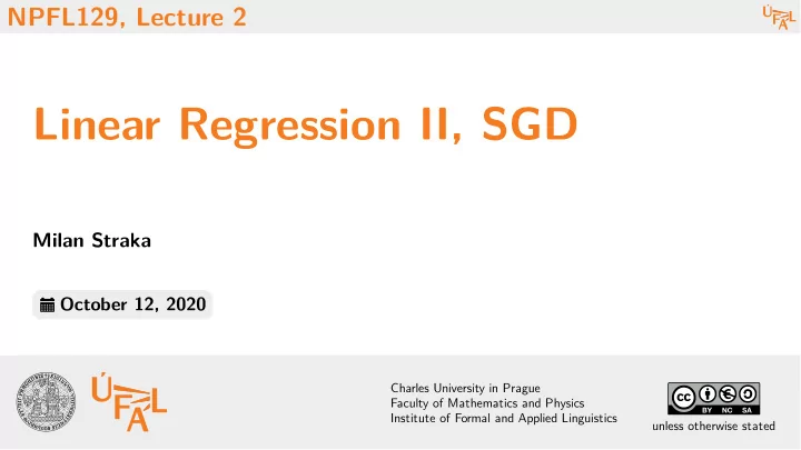
Linear Regression II, SGD Milan Straka October 12, 2020 Charles - PowerPoint PPT Presentation
NPFL129, Lecture 2 Linear Regression II, SGD Milan Straka October 12, 2020 Charles University in Prague Faculty of Mathematics and Physics Institute of Formal and Applied Linguistics unless otherwise stated Linear Regression x R D Given
NPFL129, Lecture 2 Linear Regression II, SGD Milan Straka October 12, 2020 Charles University in Prague Faculty of Mathematics and Physics Institute of Formal and Applied Linguistics unless otherwise stated
Linear Regression x ∈ R D Given an input value , linear regression computes predictions as: D ∑ y ( x ; w , b ) = x + + … + x + b = + b = x w + T b . w x w w x w 1 1 2 2 D D i i i =1 b w The bias can be considered one of the weights if convenient. We train the weights by minimizing an error function between the real target values and their predictions, notably sum of squares : N 1 ∑ 2 ( y ( x ; w ) − ) t i i 2 i =1 There are several ways how to minimize it, but in our case, there exists an explicit solution: −1 T T w = ( X X ) X t . NPFL129, Lecture 2 Refresh Regularization Hyperparameters SVD Solution Random Variables SGD LR-SGD Features 2/27
Linear Regression Example 0 1 x = ( x , x , … , x ) M ≥ 0 M Assume our input vectors comprise of , for . NPFL129, Lecture 2 Refresh Regularization Hyperparameters SVD Solution Random Variables SGD LR-SGD Features 3/27
Linear Regression Example RMSE = MSE To plot the error, the root mean squared error is frequently used. The displayed error nicely illustrates two main challenges in machine learning: underfitting overfitting NPFL129, Lecture 2 Refresh Regularization Hyperparameters SVD Solution Random Variables SGD LR-SGD Features 4/27
Model Capacity We can control whether a model underfits or overfits by modifying its capacity . representational capacity effective capacity NPFL129, Lecture 2 Refresh Regularization Hyperparameters SVD Solution Random Variables SGD LR-SGD Features 5/27
Linear Regression Overfitting Note that employing more data also usually alleviates overfitting (the relative capacity of the model is decreased). NPFL129, Lecture 2 Refresh Regularization Hyperparameters SVD Solution Random Variables SGD LR-SGD Features 6/27
Regularization Regularization in a broad sense is any change in a machine learning algorithm that is designed to reduce generalization error but not necessarily its training error). L 2 regularization (also called weighted decay) penalizes models with large weights: N 1 λ ∑ 2 2 ( y ( x ; w ) − ) + ∣∣ w ∣∣ t i i 2 2 i =1 NPFL129, Lecture 2 Refresh Regularization Hyperparameters SVD Solution Random Variables SGD LR-SGD Features 7/27
Regularizing Linear Regression In matrix form, regularized sum of squares error for linear regression amounts to 2 2 1 ∣∣ Xw − t ∣∣ + ∣∣ w ∣∣ . λ 2 2 When repeating the same calculation as in the unregularized case, we arrive at T T ( X X + λ I ) w = X t , I where is an identity matrix. X ∈ R N × D t ∈ R N λ ∈ R + Input : Dataset ( , ), constant . w ∈ R D Output : Weights minimizing MSE of regularized linear regression. −1 T T w ← ( X X + λ I ) X t . NPFL129, Lecture 2 Refresh Regularization Hyperparameters SVD Solution Random Variables SGD LR-SGD Features 8/27
Choosing Hyperparameters Hyperparameters are not adapted by the learning algorithm itself. Usually a validation set or development set is used to estimate the generalization error, allowing to update hyperparameters accordingly. If there is not enough data (well, there is always not enough data), more sophisticated approaches can be used. M λ So far, we have seen two hyperparameters, and . NPFL129, Lecture 2 Refresh Regularization Hyperparameters SVD Solution Random Variables SGD LR-SGD Features 9/27
Linear Regression When training a linear regression mode, we minimized the sum of squares error function by computing its gradient (partial derivatives with respect to all weights) and found solution when it is equal to zero, arriving at the following equation for optimal weights: X Xw = T X t . T −1 T T T w = ( X X ) X X X t If is regular, we can invert it and compute the weights as . R D × D rank( X ) = rank( X X ) T X X ∈ T If you recall that , matrix is regular if and only if X D X has rank , which is equivalent to the columns of being linearly independent. NPFL129, Lecture 2 Refresh Regularization Hyperparameters SVD Solution Random Variables SGD LR-SGD Features 10/27
SVD Solution of Linear Regression T X Xw = T T X X X t Now consider the case that is singular. We will show that is still solvable, but it does not have a unique solution. Our goal in this case will be to find ∣∣ w ∣∣ 2 w the with minimum fulfilling the equation. X = U Σ V T X We now consider singular value decomposition (SVD) of , writing , where U ∈ R N × N = [ i = j ] T u u j i is an orthogonal matrix, i.e., , Σ ∈ R N × D is a diagonal matrix, V ∈ R D × D is again an orthogonal matrix. Σ r Assuming the diagonal matrix has rank , we can write it as [ Σ 0 0 ] r Σ = , 0 R r × r Σ ∈ U V r r r r where is a regular diagonal matrix. Denoting and the matrix of first Σ T X = U U V V r r r columns of and , respectively, we can write . NPFL129, Lecture 2 Refresh Regularization Hyperparameters SVD Solution Random Variables SGD LR-SGD Features 11/27
SVD Solution of Linear Regression Σ X = U T V r r r Using the decomposition , we can rewrite the goal equation as Σ T T Σ T Σ T T w = t . V U U V V U r r r r r r r r r U r A transposition of an orthogonal matrix is its inverse. Therefore, our submatrix fulfils that T T T T = = U U I U U U U V V I r r r r r r , because is a top left submatrix of . Analogously, . We therefore simplify the goal equation to Σ Σ T Σ T w = V U t r r r r r Σ r Because the diagonal matrix is regular, we can divide by it and obtain −1 T Σ T w = t . V U r r r NPFL129, Lecture 2 Refresh Regularization Hyperparameters SVD Solution Random Variables SGD LR-SGD Features 12/27
SVD Solution of Linear Regression −1 Σ T w = T T r = D V U t X X r r r We have . If he original matrix was regular, then and V r is a square regular orthogonal matrix, in which case −1 Σ T w = V t . U r r r + −1 R D × N Σ ∈ Σ i , i If we denote the diagonal matrix with on diagonal, we can rewrite to + w = V Σ U t . T T r < D V w = y r Now if , is undetermined and has infinitely many solutions. To find the one T ∣∣ w ∣∣ V w V with smallest norm , consider the full product . Because is orthogonal, T T ∣∣ V w ∣∣ = ∣∣ w ∣∣ ∣∣ V w ∣∣ w , and it is sufficient to find with smallest . We know that the first T T ∣∣ V w ∣∣ ∣∣ V w ∣∣ r elements of are fixed by the above equation – the smallest can be + Σ U t T D − r therefore obtained by setting the last elements to zero. Finally, we note that is −1 + Σ T w = V Σ U t T D − r U t r r exactly padded with zeros, obtaining the same solution . NPFL129, Lecture 2 Refresh Regularization Hyperparameters SVD Solution Random Variables SGD LR-SGD Features 13/27
SVD Solution of Linear Regression and Pseudoinverses The solution to a linear regression with sum of squares error function is tightly connected X to matrix pseudoinverses. If a matrix is singular or rectangular, it does not have an Xw = b exact inverse, and does not have an exact solution. However, we can consider the so-called Moore-Penrose pseudoinverse X + = def V Σ U + T to be the closest approximation to an inverse, in the sense that we can find the best solution + Xw = b w = X b (with smallest MSE) to the equation by setting . X Alternatively, we can define the pseudoinverse of a matrix as + = arg min ∣∣ XY − ∣∣ = arg min ∣∣ Y X − ∣∣ X I I N F D F Y ∈ R D × N Y ∈ R N × D which can be verified to be the same as our SVD formula. NPFL129, Lecture 2 Refresh Regularization Hyperparameters SVD Solution Random Variables SGD LR-SGD Features 14/27
Random Variables x A random variable is a result of a random process. It can be discrete or continuous. Probability Distribution A probability distribution describes how likely are individual values a random variable can take. x ∼ P x P The notation stands for a random variable having a distribution . x P ( x ) x For discrete variables, the probability that takes a value is denoted as or explicitly as P (x = x ) x . All probabilities are non-negative and sum of probabilities of all possible values of P (x = x ) = 1 ∑ x is . x [ a , b ] For continuous variables, the probability that the value of lies in the interval is given by b p ( x ) d x ∫ a . NPFL129, Lecture 2 Refresh Regularization Hyperparameters SVD Solution Random Variables SGD LR-SGD Features 15/27
Random Variables Expectation f ( x ) P ( x ) The expectation of a function with respect to discrete probability distribution is defined as: ∑ E def [ f ( x )] = P ( x ) f ( x ) x∼ P x For continuous variables it is computed as: ∫ def E [ f ( x )] = p ( x ) f ( x ) d x x∼ p x E E [ x ] [ x ] P If the random variable is obvious from context, we can write only of even . Expectation is linear, i.e., E βg ( x )] = α E β E [ αf ( x ) + [ f ( x )] + [ g ( x )] x x x NPFL129, Lecture 2 Refresh Regularization Hyperparameters SVD Solution Random Variables SGD LR-SGD Features 16/27
Recommend
More recommend
Explore More Topics
Stay informed with curated content and fresh updates.
