Linear Regression II, SGD, Perceptron Milan Straka October 14, - PowerPoint PPT Presentation
NPFL129, Lecture 2 Linear Regression II, SGD, Perceptron Milan Straka October 14, 2019 Charles University in Prague Faculty of Mathematics and Physics Institute of Formal and Applied Linguistics unless otherwise stated Linear Regression x
NPFL129, Lecture 2 Linear Regression II, SGD, Perceptron Milan Straka October 14, 2019 Charles University in Prague Faculty of Mathematics and Physics Institute of Formal and Applied Linguistics unless otherwise stated
Linear Regression x ∈ R d Given an input value , one of the simplest models to predict a target real value is linear regression : d ∑ T f ( x ; w , b ) = x + + … + x + b = + b = x w + b . w x w w x w 1 1 2 2 D D i i i =1 b w The bias can be considered one of the weights if convenient. By computing derivatives of a sum of squares error function, we arrived at the following equation for the optimum weights: T T X Xw = X t . −1 T w = ( X X ) T T X X X t If is regular, we can invert it and compute the weights as . T X X X d X Matrix is regular if and only if has rank , which is equivalent to the columns of being linearly independent. NPFL129, Lecture 2 Regression Random Variables SGD Features CV Perceptron 2/23
SVD Solution of Linear Regression T X Xw = T T X X X t Now consider the case that is singular. We will show that is still solvable, but it does not have a unique solution. Our goal in this case will be to find w the smallest fulfilling the equation. X = UΣV T We now consider singular value decomposition (SVD) of X, writing , where U ∈ R N × N = [ i = j ] T u u j i is an orthogonal matrix, i.e., , Σ ∈ R N × D is a diagonal matrix, V ∈ R D × D is again an orthogonal matrix. Σ r Assuming the diagonal matrix has rank , we can write it as 0 [ Σ 0 ] r Σ = , 0 R d × d ∈ Σ U V r r r r where is a regular diagonal matrix. Denoting and the matrix of first T X = U U V Σ V r r r columns of and , respectively, we can write . NPFL129, Lecture 2 Regression Random Variables SGD Features CV Perceptron 3/23
SVD Solution of Linear Regression X = U T Σ V r r r Using the decomposition , we can rewrite the goal equation as T T T T T w = t . V Σ U U Σ V V Σ U r r r r r r r r r U r A transposition of an orthogonal matrix is its inverse. Therefore, our submatrix fulfils that T T T T = = U U I U U U U V V I r r r r r r , because is a top left submatrix of . Analogously, . We therefore simplify the goal equation to T T w = Σ Σ V Σ U t r r r r r Σ r Because the diagonal matrix is regular, we can divide by it and obtain −1 T T w = t . V Σ U r r r NPFL129, Lecture 2 Regression Random Variables SGD Features CV Perceptron 4/23
SVD Solution of Linear Regression −1 T w = T T r = d V Σ U t X X r r r We have . If he original matrix was regular, then and V r is a square regular orthogonal matrix, in which case −1 T w = V t . Σ U r r r + −1 R D × N ∈ Σ Σ i , i If we denote the diagonal matrix with on diagonal, we can rewrite to + T w = V Σ U t . T r < d V w = y r Now if , is undetermined and has infinitely many solutions. To find the one T ∣∣ w ∣∣ V w V with smallest norm , consider the full product . Because is orthogonal, T T ∣∣ V w ∣∣ = ∣∣ w ∣∣ ∣∣ V w ∣∣ w , and it is sufficient to find with smallest . We know that the first T T ∣∣ V w ∣∣ ∣∣ V w ∣∣ r elements of are fixed by the above equation – the smallest can be + T d − r Σ U t therefore obtained by setting the last elements to zero. Finally, we note that is −1 + T T d − r w = V Σ U t Σ U t r r exactly padded with zeros, obtaining the same solution . NPFL129, Lecture 2 Regression Random Variables SGD Features CV Perceptron 5/23
SVD Solution of Linear Regression and Pseudoinverses The solution to a linear regression with sum of squares error function is tightly connected X to matrix pseudoinverses. If a matrix is singular or rectangular, it does not have an Xw = b exact inverse, and does not have an exact solution. However, we can consider the so-called Moore-Penrose pseudoinverse X + = def V Σ U + T to be the closest approximation to an inverse, in the sense that we can find the best solution + Xw = b w = X b (with smallest MSE) to the equation by setting . Alternatively, we can define the pseudoinverse as + = arg min ∣∣ XY − ∣∣ = arg min ∣∣ Y X − ∣∣ X I I N F D F Y ∈ R D × N Y ∈ R N × D which can be verified to be the same as our SVD formula. NPFL129, Lecture 2 Regression Random Variables SGD Features CV Perceptron 6/23
Random Variables x A random variable is a result of a random process. It can be discrete or continuous. Probability Distribution A probability distribution describes how likely are individual values a random variable can take. x ∼ P x P The notation stands for a random variable having a distribution . x P ( x ) x For discrete variables, the probability that takes a value is denoted as or explicitly as P (x = x ) x . All probabilities are non-negative and sum of probabilities of all possible values of P (x = x ) = 1 ∑ x is . x [ a , b ] For continuous variables, the probability that the value of lies in the interval is given by b p ( x ) d x ∫ a . NPFL129, Lecture 2 Regression Random Variables SGD Features CV Perceptron 7/23
Random Variables Expectation f ( x ) P ( x ) The expectation of a function with respect to discrete probability distribution is defined as: ∑ E def [ f ( x )] = P ( x ) f ( x ) x∼ P x For continuous variables it is computed as: ∫ def E [ f ( x )] = p ( x ) f ( x ) d x x∼ p x E E [ x ] [ x ] P If the random variable is obvious from context, we can write only of even . Expectation is linear, i.e., E βg ( x )] = α E β E [ αf ( x ) + [ f ( x )] + [ g ( x )] x x x NPFL129, Lecture 2 Regression Random Variables SGD Features CV Perceptron 8/23
Random Variables Variance μ = E [ x ] Variance measures how much the values of a random variable differ from its mean . [ 2 ] def E ( x − E [ x ] ) Var( x ) = , or more generally [ 2 ] def E ( f ( x ) − E [ f ( x )] ) Var( f ( x )) = It is easy to see that [ 2 2 ] 2 2 ] Var( x ) = E x − 2 x E [ x ] + ( E [ x ] ) E x ( E [ x ] ) , = − [ E [ 2 x E [ x ] ] = 2( E [ x ]) 2 because . 2 E [ x ] Variance is connected to , a second moment of a random variable – it is in fact a centered second moment. NPFL129, Lecture 2 Regression Random Variables SGD Features CV Perceptron 9/23
Estimators and Bias An estimator is a rule for computing an estimate of a given value, often an expectation of some random value(s). For example, we might estimate mean of random variable by sampling a value according to its probability distribution. Bias of an estimator is the difference of the expected value of the estimator and the true value being estimated: bias = E [estimate] − true estimated value. If the bias is zero, we call the estimator unbiased , otherwise we call it biased . NPFL129, Lecture 2 Regression Random Variables SGD Features CV Perceptron 10/23
Estimators and Bias If we have a sequence of estimates, it also might happen that the bias converges to zero. x , … , x 1 n Consider the well known sample estimate of variance. Given independent and identically distributed random variables, we might estimate mean and variance as 1 ∑ 1 ∑ ^ 2 ^ = , ^ 2 = ( x − ) . μ x σ μ i i n n i i E [ 1 ^ 2 2 ] = (1 − ) σ σ n Such estimate is biased, because , but the bias converges to zero with n increasing . Also, an unbiased estimator does not necessarily have small variance – in some cases it can have large variance, so a biased estimator with smaller variance might be preferred. NPFL129, Lecture 2 Regression Random Variables SGD Features CV Perceptron 11/23
Gradient Descent Sometimes it is more practical to search for the best model weights in an iterative/incremental/sequential fashion. Either because there is too much data, or the direct optimization is not feasible. Assuming we are minimizing an error function arg min E ( w ), w we may use gradient descent : w ← w − α ∇ E ( w ) w α The constant is called a learning rate and specifies the “ length ” of a step we perform in every iteration of the gradient descent. Figure 4.1, page 83 of Deep Learning Book, http://deeplearningbook.org NPFL129, Lecture 2 Regression Random Variables SGD Features CV Perceptron 12/23
Gradient Descent Variants Consider an error function computed as an expectation over the dataset: E ∇ E ( w ) = ∇ L ( f ( x ; w ), t ) . ( x , t )∼ ^ data w w p ∇ E ( w ) w (Regular) Gradient Descent : We use all training data to compute exactly. ∇ E ( w ) w Online (or Stochastic) Gradient Descent : We estimate using a single random example from the training data. Such an estimate is unbiased, but very noisy. ∇ E ( w ) ≈ ∇ L ( f ( x ; w ), t ) for randomly chosen ( x , t ) from ^ data . p w w Minibatch SGD : The minibatch SGD is a trade-off between gradient descent and SGD – ∇ E ( w ) m w the expectation in is estimated using random independent examples from the training data. m 1 ∑ ∇ E ( w ) ≈ ∇ L ( f ( x ; w ), t ) for randomly chosen ( x , t ) from ^ data . p w w i i i i m i =1 NPFL129, Lecture 2 Regression Random Variables SGD Features CV Perceptron 13/23
Recommend
More recommend
Explore More Topics
Stay informed with curated content and fresh updates.
