SGD and Averaging Instructor: Sham Kakade 1 SGD and optimality - PDF document
CSE 547/Stat 548: Machine Learning for Big Data Lecture SGD and Averaging Instructor: Sham Kakade 1 SGD and optimality There is a strong sense in which SGD can be made optimal, if we perform averaging. SGD itself is really not optimal,
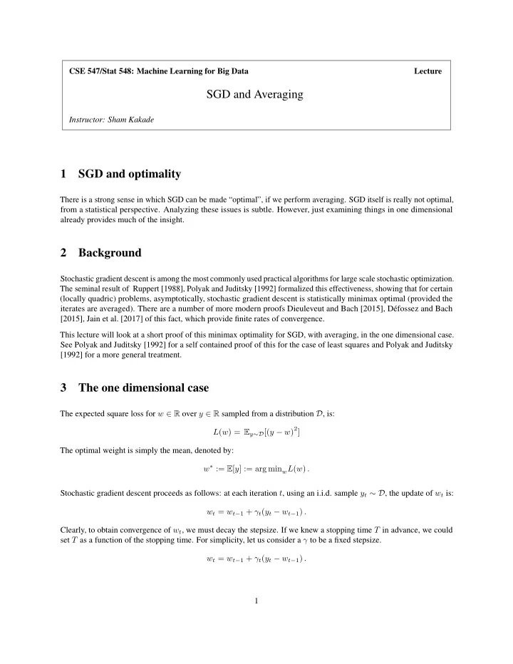
CSE 547/Stat 548: Machine Learning for Big Data Lecture SGD and Averaging Instructor: Sham Kakade 1 SGD and optimality There is a strong sense in which SGD can be made “optimal”, if we perform averaging. SGD itself is really not optimal, from a statistical perspective. Analyzing these issues is subtle. However, just examining things in one dimensional already provides much of the insight. 2 Background Stochastic gradient descent is among the most commonly used practical algorithms for large scale stochastic optimization. The seminal result of Ruppert [1988], Polyak and Juditsky [1992] formalized this effectiveness, showing that for certain (locally quadric) problems, asymptotically, stochastic gradient descent is statistically minimax optimal (provided the iterates are averaged). There are a number of more modern proofs Dieuleveut and Bach [2015], Défossez and Bach [2015], Jain et al. [2017] of this fact, which provide finite rates of convergence. This lecture will look at a short proof of this minimax optimality for SGD, with averaging, in the one dimensional case. See Polyak and Juditsky [1992] for a self contained proof of this for the case of least squares and Polyak and Juditsky [1992] for a more general treatment. 3 The one dimensional case The expected square loss for w ∈ R over y ∈ R sampled from a distribution D , is: L ( w ) = E y ∼D [( y − w ) 2 ] The optimal weight is simply the mean, denoted by: w ∗ := E [ y ] := arg min w L ( w ) . Stochastic gradient descent proceeds as follows: at each iteration t , using an i.i.d. sample y t ∼ D , the update of w t is: w t = w t − 1 + γ t ( y t − w t − 1 ) . Clearly, to obtain convergence of w t , we must decay the stepsize. If we knew a stopping time T in advance, we could set T as a function of the stopping time. For simplicity, let us consider a γ to be a fixed stepsize. w t = w t − 1 + γ t ( y t − w t − 1 ) . 1
The statistically optimal rate. Using n samples (and for large enough n ), the minimax optimal rate is achieved by the sample mean (more generally, the maximum likelihood estimator, or, equivalently, the empirical risk minimizer). Denote the variance as: � ( y − E [ y ]) 2 � σ 2 := E . Given n i.i.d. samples { ( y i ) } n i =1 , the best estimator is sample mean: n � := 1 1 2 ( y i − w · x i ) 2 . w SampMean � n n i =1 This optimal (among estimators) is characterized as follows: )] − L ( w ∗ ) = σ 2 w SampMean E [ L ( � n n 4 SGD itself isn’t all that great... This is a little surprising, that even in one dimension, SGD doesn’t really get it right. SGD with a constant learning rate. Define the noise in iteration t (of the t -th sample) as: ǫ t := E [ y ] − y t , which is a mean 0 quantity. The SGD rule can be written as: w t − w ∗ = w t − 1 − w ∗ + γ ( y t − w t − 1 ) = (1 − γ )( w t − 1 − w ∗ ) − γǫ t . Roughly speaking, the above shows how the process on w t − w ∗ consists of a contraction along with an addition of a zero mean quantity. From recursion, � � w t − w ∗ = (1 − γ ) t ( w 0 − w ∗ ) − γ ǫ t + (1 − γ ) ǫ t − 1 + · · · + (1 − γ ) t ǫ 1 . Lemma 4.1. We have that: t − 1 � E [ L ( w t )] − L ( w ∗ ) = E [( w t − w ∗ ) 2 ] = (1 − γ ) t ( w 0 − w ∗ ) 2 + γ 2 σ 2 (1 − γ ) 2 t τ =0 ≤ exp ( − γt )( w 0 − w ∗ ) 2 + γσ 2 . Proof. That E [ L ( w t ) − L ( w ∗ ) = E [( w t − w ∗ ) 2 ] is straight forward. To prove the equality, we note that the noise is mean 0 , i.e. E [ ǫ t ] = 0 , and the noise is independent, so E [ ǫ t ǫ t ′ ] = 0 for t � = t ′ . Hence, we have that: E [( w t − w ∗ ) 2 ] = (1 − γ ) t ( w 0 − w ∗ ) − γ 2 � σ 2 + (1 − γ ) 2 σ 2 + · · · + (1 − γ ) 2 t σ 2 � . . which leads to the first claim. The last step simply follows from summing the geometric series, to obtain: t − 1 � γ 2 γ 2 (1 − γ ) t ≤ γ 2 1 − (1 − γ ) 2 ≤ 1 − (1 − γ ) = γ τ =0 which completes the proof. 2
There is no good choice of a learning rate. We would ideally hope for a rate that (eventually) matches σ 2 /n which is the rate of the sample average. Note that our derivation is exact (the only step with an inequality is summing the geometric series, which is looses very little). Let us try out a few learning rates to get intuition. Let us consider γ = 1 / 2 . (let’s rule out γ = 1 , as we jump to the 0 bias in one step. This does not hold for other problems, e.g. in more than one dimension such as for regression.) Here we have: E [( w t − w ∗ ) 2 ] ≤ exp ( − t/ 2)( w 0 − w ∗ ) 2 + σ 2 2 . The first term (the bias) is dropping extremely quickly (geometrically). The variance is not even going to 0 , so, of course, this is extremely poor. √ Setting η = 1 / t , we have: √ t )( w 0 − w ∗ ) 2 + σ 2 E [( w t − w ∗ ) 2 ] ≤ exp ( − √ t . which at least goes to 0 . However, the bias term is dropping much more slowly than before, and the variance term, while going to 0 , is much worse than the rate of the sample average! Now, let us look at η = 1 /T . Here we have: E [( w t − w ∗ ) 2 ] ≤ exp ( − 1)( w 0 − w ∗ ) 2 + σ 2 t . Here, the variance term is in fact dropping at the optimal rate. However, the bias term does not even go 0 , so, overal, this is another extremely poor choice. Is there really no choice of time varying learning rate?. One may hope to instead try a decaying learning scheme, where we set γ t and decay it over time (rather than just setting as a function of the stopping time). This does not improve things (though a decaying γ as O (1 /t ) does improve upon the previous bounds). The reader might not that restart scheme will work here, if one thinks this through. More generally (if we move to regression), there is in fact no decaying learning rate scheme which is optimal (one can prove a lower bound on this); meaning that the statistical minimax rate will not be reached. 5 Iterate Averaging Remarkably, an extremely procedure will give us the best of both worlds, where our bias drops geometrically and the variance is optimal (to within a constant). The approach is extremely effective even in non-convex settings. The iterate averaging algorithm does not actually change SGD algorithm. Instead, you just keep track of a running average of your w t ’s (say starting at some point in time) and you use that instead of using the last point w t . Note that you still just run your usual SGD algorithm as you were doing before! Denote the average iterate, averaged from iteration t to T , by: T − 1 � 1 w t ′ . w t : T := T − t t ′ = t Note there is a choice of when to start averaging. In practice, we often cycle through our dataset. 3
Theorem 5.1. Suppose γ < 1 / 2 . The risk is bounded as: � − t/ 2)( w 0 − w ∗ ) 2 + 4 σ 2 E [( w t : T − w ∗ ) 2 ] ≤ 2 exp ( T − t . For t = T/ 2 , i.e. we start our average over the second half of the samples, we have: � − T/ 4)( w 0 − w ∗ ) 2 + 8 σ 2 E [( w T/ 2: T − w ∗ ) 2 ] ≤ 2 exp ( T . We have that, with iterate averaging, the bias term (the first term) decays at a geometric rate, and the variance term is withint a constant factor of the optimal variance (we have not optimized this constant). Also, even if did not know T in advance, it is easy enough to maintain multiple running averages (or restart the running average). Thus, iterative averaging gives the best of both worlds! And this phenomena seems to far more general. Empirically, it also works very well in non-convex cases. This theorem is really a simple special case of results in the literature, e.g. see Jain et al. [2017]. It is not particularly difficult to prove in the 1 -dimensional case. References Alexandre Défossez and Francis R. Bach. Averaged least-mean-squares: Bias-variance trade-offs and optimal sampling distributions. In AISTATS , volume 38, 2015. Aymeric Dieuleveut and Francis R. Bach. Non-parametric stochastic approximation with large step sizes. The Annals of Statistics , 2015. P. Jain, S. Kakade, R. Kidambi, P. Netrapalli, and V. Pillutla andA. Sidford. A markov chain theory approach to characterizing the minimax optimality of stochastic gradient descent (for least squares). In 37th Foundations of Software Technology and Theoretical Computer Science, 2017 , 2017. Boris T. Polyak and Anatoli B. Juditsky. Acceleration of stochastic approximation by averaging. SIAM Journal on Control and Optimization , volume 30, 1992. David Ruppert. Efficient estimations from a slowly convergent robbins-monro process. Tech. Report, ORIE, Cornell University , 1988. 4
Recommend
More recommend
Explore More Topics
Stay informed with curated content and fresh updates.
