Forecasting Ination Using Dynamic Model Averaging Gary Koop and - PowerPoint PPT Presentation
Forecasting Ination Using Dynamic Model Averaging Gary Koop and Dimitris Korobilis September 20, 2010 Gary Koop and Dimitris Korobilis () Dynamic Model Averaging September 20, 2010 1 / 33 Introduction Macroeconomists typically have many
Consider forecasting y τ + 1 . Recursive forecasting methods: b θ = estimate using data through τ . So b θ will change (a bit) with τ , but can change too slowly Rolling forecasts use: b θ an estimate using data from τ � τ 0 through τ . Better at capturing parameter change, but need to choose τ 0 Recursive and rolling forecasts might be imperfect solutions Gary Koop and Dimitris Korobilis () Dynamic Model Averaging September 20, 2010 8 / 33
Consider forecasting y τ + 1 . Recursive forecasting methods: b θ = estimate using data through τ . So b θ will change (a bit) with τ , but can change too slowly Rolling forecasts use: b θ an estimate using data from τ � τ 0 through τ . Better at capturing parameter change, but need to choose τ 0 Recursive and rolling forecasts might be imperfect solutions Why not use a model which formally models the parameter change as well? Gary Koop and Dimitris Korobilis () Dynamic Model Averaging September 20, 2010 8 / 33
Time Varying Parameter (TVP) Models TVP models gaining popularity in empirical macroeconomics = z t θ t + ε t y t θ t = θ t � 1 + η t Gary Koop and Dimitris Korobilis () Dynamic Model Averaging September 20, 2010 9 / 33
Time Varying Parameter (TVP) Models TVP models gaining popularity in empirical macroeconomics = z t θ t + ε t y t θ t = θ t � 1 + η t ind � N ( 0 , H t ) ε t Gary Koop and Dimitris Korobilis () Dynamic Model Averaging September 20, 2010 9 / 33
Time Varying Parameter (TVP) Models TVP models gaining popularity in empirical macroeconomics = z t θ t + ε t y t θ t = θ t � 1 + η t ind � N ( 0 , H t ) ε t ind � N ( 0 , Q t ) η t Gary Koop and Dimitris Korobilis () Dynamic Model Averaging September 20, 2010 9 / 33
Time Varying Parameter (TVP) Models TVP models gaining popularity in empirical macroeconomics = z t θ t + ε t y t θ t = θ t � 1 + η t ind � N ( 0 , H t ) ε t ind � N ( 0 , Q t ) η t Standard statistical methods (e.g. involving Kalman …lter and state smoother) exist for them Gary Koop and Dimitris Korobilis () Dynamic Model Averaging September 20, 2010 9 / 33
Why not use TVP model to forecast in‡ation? Gary Koop and Dimitris Korobilis () Dynamic Model Averaging September 20, 2010 10 / 33
Why not use TVP model to forecast in‡ation? Advantage: models parameter change in a formal manner Gary Koop and Dimitris Korobilis () Dynamic Model Averaging September 20, 2010 10 / 33
Why not use TVP model to forecast in‡ation? Advantage: models parameter change in a formal manner Disadvantage: same predictors used at all points in time. Gary Koop and Dimitris Korobilis () Dynamic Model Averaging September 20, 2010 10 / 33
Why not use TVP model to forecast in‡ation? Advantage: models parameter change in a formal manner Disadvantage: same predictors used at all points in time. If number of predictors large, over-…t, over-parameterization problems Gary Koop and Dimitris Korobilis () Dynamic Model Averaging September 20, 2010 10 / 33
Why not use TVP model to forecast in‡ation? Advantage: models parameter change in a formal manner Disadvantage: same predictors used at all points in time. If number of predictors large, over-…t, over-parameterization problems In our empirical work, we show very poor forecast performance Gary Koop and Dimitris Korobilis () Dynamic Model Averaging September 20, 2010 10 / 33
Why not use TVP model to forecast in‡ation? Advantage: models parameter change in a formal manner Disadvantage: same predictors used at all points in time. If number of predictors large, over-…t, over-parameterization problems In our empirical work, we show very poor forecast performance Bayesian model averaging methods popular way of addressing this problem in cross-sectional regression Gary Koop and Dimitris Korobilis () Dynamic Model Averaging September 20, 2010 10 / 33
Why not use TVP model to forecast in‡ation? Advantage: models parameter change in a formal manner Disadvantage: same predictors used at all points in time. If number of predictors large, over-…t, over-parameterization problems In our empirical work, we show very poor forecast performance Bayesian model averaging methods popular way of addressing this problem in cross-sectional regression How to adapt BMA to TVP models? Gary Koop and Dimitris Korobilis () Dynamic Model Averaging September 20, 2010 10 / 33
Dynamic Model Averaging (DMA) De…ne K models which have z ( k ) for k = 1 , .., K , as predictors t Gary Koop and Dimitris Korobilis () Dynamic Model Averaging September 20, 2010 11 / 33
Dynamic Model Averaging (DMA) De…ne K models which have z ( k ) for k = 1 , .., K , as predictors t z ( k ) is subset of z t . t Gary Koop and Dimitris Korobilis () Dynamic Model Averaging September 20, 2010 11 / 33
Dynamic Model Averaging (DMA) De…ne K models which have z ( k ) for k = 1 , .., K , as predictors t z ( k ) is subset of z t . t Set of models: z ( k ) θ ( k ) + ε ( k ) = y t t t t θ ( k ) θ ( k ) + η ( k ) = t + 1 t t Gary Koop and Dimitris Korobilis () Dynamic Model Averaging September 20, 2010 11 / 33
Dynamic Model Averaging (DMA) De…ne K models which have z ( k ) for k = 1 , .., K , as predictors t z ( k ) is subset of z t . t Set of models: z ( k ) θ ( k ) + ε ( k ) = y t t t t θ ( k ) θ ( k ) + η ( k ) = t + 1 t t � � ε ( k ) 0 , H ( k ) is N t t Gary Koop and Dimitris Korobilis () Dynamic Model Averaging September 20, 2010 11 / 33
Dynamic Model Averaging (DMA) De…ne K models which have z ( k ) for k = 1 , .., K , as predictors t z ( k ) is subset of z t . t Set of models: z ( k ) θ ( k ) + ε ( k ) = y t t t t θ ( k ) θ ( k ) + η ( k ) = t + 1 t t � � ε ( k ) 0 , H ( k ) is N t t � � η ( k ) 0 , Q ( k ) is N t t Gary Koop and Dimitris Korobilis () Dynamic Model Averaging September 20, 2010 11 / 33
Dynamic Model Averaging (DMA) De…ne K models which have z ( k ) for k = 1 , .., K , as predictors t z ( k ) is subset of z t . t Set of models: z ( k ) θ ( k ) + ε ( k ) = y t t t t θ ( k ) θ ( k ) + η ( k ) = t + 1 t t � � ε ( k ) 0 , H ( k ) is N t t � � η ( k ) 0 , Q ( k ) is N t t Let L t 2 f 1 , 2 , .., K g denote which model applies at t Gary Koop and Dimitris Korobilis () Dynamic Model Averaging September 20, 2010 11 / 33
Why not just forecast using BMA over these TVP models at every point in time? Gary Koop and Dimitris Korobilis () Dynamic Model Averaging September 20, 2010 12 / 33
Why not just forecast using BMA over these TVP models at every point in time? Di¤erent weights in averaging at every point in time. Gary Koop and Dimitris Korobilis () Dynamic Model Averaging September 20, 2010 12 / 33
Why not just forecast using BMA over these TVP models at every point in time? Di¤erent weights in averaging at every point in time. Or why not just select a single TVP forecasting model at every point in time? Gary Koop and Dimitris Korobilis () Dynamic Model Averaging September 20, 2010 12 / 33
Why not just forecast using BMA over these TVP models at every point in time? Di¤erent weights in averaging at every point in time. Or why not just select a single TVP forecasting model at every point in time? Di¤erent forecasting models selected at each point in time. Gary Koop and Dimitris Korobilis () Dynamic Model Averaging September 20, 2010 12 / 33
Why not just forecast using BMA over these TVP models at every point in time? Di¤erent weights in averaging at every point in time. Or why not just select a single TVP forecasting model at every point in time? Di¤erent forecasting models selected at each point in time. If K is large (e.g. K = 2 m ), this is computationally infeasible. Gary Koop and Dimitris Korobilis () Dynamic Model Averaging September 20, 2010 12 / 33
Why not just forecast using BMA over these TVP models at every point in time? Di¤erent weights in averaging at every point in time. Or why not just select a single TVP forecasting model at every point in time? Di¤erent forecasting models selected at each point in time. If K is large (e.g. K = 2 m ), this is computationally infeasible. With cross-sectional BMA have to work with model space K = 2 m which is computationally burdensome Gary Koop and Dimitris Korobilis () Dynamic Model Averaging September 20, 2010 12 / 33
Why not just forecast using BMA over these TVP models at every point in time? Di¤erent weights in averaging at every point in time. Or why not just select a single TVP forecasting model at every point in time? Di¤erent forecasting models selected at each point in time. If K is large (e.g. K = 2 m ), this is computationally infeasible. With cross-sectional BMA have to work with model space K = 2 m which is computationally burdensome In present time series context, forecasting through time τ involves 2 m τ models. Gary Koop and Dimitris Korobilis () Dynamic Model Averaging September 20, 2010 12 / 33
Why not just forecast using BMA over these TVP models at every point in time? Di¤erent weights in averaging at every point in time. Or why not just select a single TVP forecasting model at every point in time? Di¤erent forecasting models selected at each point in time. If K is large (e.g. K = 2 m ), this is computationally infeasible. With cross-sectional BMA have to work with model space K = 2 m which is computationally burdensome In present time series context, forecasting through time τ involves 2 m τ models. Also, Bayesian inference in TVP model requires MCMC (unlike cross-sectional regression). Computationally burdensome. Gary Koop and Dimitris Korobilis () Dynamic Model Averaging September 20, 2010 12 / 33
Why not just forecast using BMA over these TVP models at every point in time? Di¤erent weights in averaging at every point in time. Or why not just select a single TVP forecasting model at every point in time? Di¤erent forecasting models selected at each point in time. If K is large (e.g. K = 2 m ), this is computationally infeasible. With cross-sectional BMA have to work with model space K = 2 m which is computationally burdensome In present time series context, forecasting through time τ involves 2 m τ models. Also, Bayesian inference in TVP model requires MCMC (unlike cross-sectional regression). Computationally burdensome. Even clever algorithms like MC-cubed are not good enough to handle this. Gary Koop and Dimitris Korobilis () Dynamic Model Averaging September 20, 2010 12 / 33
Another strategy has been used to deal with similar problems in di¤erent contexts (e.g. multiple structural breaks): Markov switching Gary Koop and Dimitris Korobilis () Dynamic Model Averaging September 20, 2010 13 / 33
Another strategy has been used to deal with similar problems in di¤erent contexts (e.g. multiple structural breaks): Markov switching Markov transition matrix, P , Gary Koop and Dimitris Korobilis () Dynamic Model Averaging September 20, 2010 13 / 33
Another strategy has been used to deal with similar problems in di¤erent contexts (e.g. multiple structural breaks): Markov switching Markov transition matrix, P , Elements p ij = Pr ( L t = i j L t � 1 = j ) for i , j = 1 , .., K . Gary Koop and Dimitris Korobilis () Dynamic Model Averaging September 20, 2010 13 / 33
Another strategy has been used to deal with similar problems in di¤erent contexts (e.g. multiple structural breaks): Markov switching Markov transition matrix, P , Elements p ij = Pr ( L t = i j L t � 1 = j ) for i , j = 1 , .., K . “If j is the forecasting model at t � 1, we switch to forecasting model i at time t with probability p ij " Gary Koop and Dimitris Korobilis () Dynamic Model Averaging September 20, 2010 13 / 33
Another strategy has been used to deal with similar problems in di¤erent contexts (e.g. multiple structural breaks): Markov switching Markov transition matrix, P , Elements p ij = Pr ( L t = i j L t � 1 = j ) for i , j = 1 , .., K . “If j is the forecasting model at t � 1, we switch to forecasting model i at time t with probability p ij " Bayesian inference is theoretically straightforward, but computationally infeasible Gary Koop and Dimitris Korobilis () Dynamic Model Averaging September 20, 2010 13 / 33
Another strategy has been used to deal with similar problems in di¤erent contexts (e.g. multiple structural breaks): Markov switching Markov transition matrix, P , Elements p ij = Pr ( L t = i j L t � 1 = j ) for i , j = 1 , .., K . “If j is the forecasting model at t � 1, we switch to forecasting model i at time t with probability p ij " Bayesian inference is theoretically straightforward, but computationally infeasible P is K � K : an enormous matrix. Gary Koop and Dimitris Korobilis () Dynamic Model Averaging September 20, 2010 13 / 33
Another strategy has been used to deal with similar problems in di¤erent contexts (e.g. multiple structural breaks): Markov switching Markov transition matrix, P , Elements p ij = Pr ( L t = i j L t � 1 = j ) for i , j = 1 , .., K . “If j is the forecasting model at t � 1, we switch to forecasting model i at time t with probability p ij " Bayesian inference is theoretically straightforward, but computationally infeasible P is K � K : an enormous matrix. Even if computation were possible, imprecise estimation of so many parameters Gary Koop and Dimitris Korobilis () Dynamic Model Averaging September 20, 2010 13 / 33
Solution: DMA Adopt approach used by Raftery et al (2007 working paper) in an engineering application Gary Koop and Dimitris Korobilis () Dynamic Model Averaging September 20, 2010 14 / 33
Solution: DMA Adopt approach used by Raftery et al (2007 working paper) in an engineering application Involves two approximations Gary Koop and Dimitris Korobilis () Dynamic Model Averaging September 20, 2010 14 / 33
Solution: DMA Adopt approach used by Raftery et al (2007 working paper) in an engineering application Involves two approximations First approximation means we do not need MCMC in each TVP model (only Kalman …ltering and smoothing) Gary Koop and Dimitris Korobilis () Dynamic Model Averaging September 20, 2010 14 / 33
Solution: DMA Adopt approach used by Raftery et al (2007 working paper) in an engineering application Involves two approximations First approximation means we do not need MCMC in each TVP model (only Kalman …ltering and smoothing) See paper for details. Idea: replace Q ( k ) and H ( k ) by estimates t t Gary Koop and Dimitris Korobilis () Dynamic Model Averaging September 20, 2010 14 / 33
Sketch of some Kalman …ltering ideas (where y t � 1 are observations through t � 1) � � θ t � 1 j y t � 1 � N b θ t � 1 , Σ t � 1 j t � 1 Gary Koop and Dimitris Korobilis () Dynamic Model Averaging September 20, 2010 15 / 33
Sketch of some Kalman …ltering ideas (where y t � 1 are observations through t � 1) � � θ t � 1 j y t � 1 � N b θ t � 1 , Σ t � 1 j t � 1 Textbook formula for b θ t � 1 and Σ t � 1 j t � 1 Gary Koop and Dimitris Korobilis () Dynamic Model Averaging September 20, 2010 15 / 33
Sketch of some Kalman …ltering ideas (where y t � 1 are observations through t � 1) � � θ t � 1 j y t � 1 � N b θ t � 1 , Σ t � 1 j t � 1 Textbook formula for b θ t � 1 and Σ t � 1 j t � 1 Then update � � θ t j y t � 1 � N b θ t � 1 , Σ t j t � 1 Gary Koop and Dimitris Korobilis () Dynamic Model Averaging September 20, 2010 15 / 33
Sketch of some Kalman …ltering ideas (where y t � 1 are observations through t � 1) � � θ t � 1 j y t � 1 � N b θ t � 1 , Σ t � 1 j t � 1 Textbook formula for b θ t � 1 and Σ t � 1 j t � 1 Then update � � θ t j y t � 1 � N b θ t � 1 , Σ t j t � 1 Σ t j t � 1 = Σ t � 1 j t � 1 + Q t Gary Koop and Dimitris Korobilis () Dynamic Model Averaging September 20, 2010 15 / 33
Sketch of some Kalman …ltering ideas (where y t � 1 are observations through t � 1) � � θ t � 1 j y t � 1 � N b θ t � 1 , Σ t � 1 j t � 1 Textbook formula for b θ t � 1 and Σ t � 1 j t � 1 Then update � � θ t j y t � 1 � N b θ t � 1 , Σ t j t � 1 Σ t j t � 1 = Σ t � 1 j t � 1 + Q t Get rid of Q t by approximating: Σ t j t � 1 = 1 λ Σ t � 1 j t � 1 Gary Koop and Dimitris Korobilis () Dynamic Model Averaging September 20, 2010 15 / 33
Sketch of some Kalman …ltering ideas (where y t � 1 are observations through t � 1) � � θ t � 1 j y t � 1 � N b θ t � 1 , Σ t � 1 j t � 1 Textbook formula for b θ t � 1 and Σ t � 1 j t � 1 Then update � � θ t j y t � 1 � N b θ t � 1 , Σ t j t � 1 Σ t j t � 1 = Σ t � 1 j t � 1 + Q t Get rid of Q t by approximating: Σ t j t � 1 = 1 λ Σ t � 1 j t � 1 0 < λ � 1 is forgetting factor Gary Koop and Dimitris Korobilis () Dynamic Model Averaging September 20, 2010 15 / 33
Forgetting factors like this have long been used in state space literature Gary Koop and Dimitris Korobilis () Dynamic Model Averaging September 20, 2010 16 / 33
Forgetting factors like this have long been used in state space literature Implies that observations j periods in the past have weight λ j . Gary Koop and Dimitris Korobilis () Dynamic Model Averaging September 20, 2010 16 / 33
Forgetting factors like this have long been used in state space literature Implies that observations j periods in the past have weight λ j . 1 Or e¤ective window size of 1 � λ . Gary Koop and Dimitris Korobilis () Dynamic Model Averaging September 20, 2010 16 / 33
Forgetting factors like this have long been used in state space literature Implies that observations j periods in the past have weight λ j . 1 Or e¤ective window size of 1 � λ . Choose value of λ near one Gary Koop and Dimitris Korobilis () Dynamic Model Averaging September 20, 2010 16 / 33
Forgetting factors like this have long been used in state space literature Implies that observations j periods in the past have weight λ j . 1 Or e¤ective window size of 1 � λ . Choose value of λ near one λ = 0 . 99: observations …ve years ago � 80% as much weight as last period’s observation. Gary Koop and Dimitris Korobilis () Dynamic Model Averaging September 20, 2010 16 / 33
Forgetting factors like this have long been used in state space literature Implies that observations j periods in the past have weight λ j . 1 Or e¤ective window size of 1 � λ . Choose value of λ near one λ = 0 . 99: observations …ve years ago � 80% as much weight as last period’s observation. λ = 0 . 95: observations …ve years ago � 35% as much weight as last period’s observations. Gary Koop and Dimitris Korobilis () Dynamic Model Averaging September 20, 2010 16 / 33
Forgetting factors like this have long been used in state space literature Implies that observations j periods in the past have weight λ j . 1 Or e¤ective window size of 1 � λ . Choose value of λ near one λ = 0 . 99: observations …ve years ago � 80% as much weight as last period’s observation. λ = 0 . 95: observations …ve years ago � 35% as much weight as last period’s observations. We focus on λ 2 [ 0 . 95 , 1 . 00 ] . Gary Koop and Dimitris Korobilis () Dynamic Model Averaging September 20, 2010 16 / 33
Forgetting factors like this have long been used in state space literature Implies that observations j periods in the past have weight λ j . 1 Or e¤ective window size of 1 � λ . Choose value of λ near one λ = 0 . 99: observations …ve years ago � 80% as much weight as last period’s observation. λ = 0 . 95: observations …ve years ago � 35% as much weight as last period’s observations. We focus on λ 2 [ 0 . 95 , 1 . 00 ] . If λ = 1 no time variation in parameters (standard recursive forecasting) Gary Koop and Dimitris Korobilis () Dynamic Model Averaging September 20, 2010 16 / 33
Forgetting factors like this have long been used in state space literature Implies that observations j periods in the past have weight λ j . 1 Or e¤ective window size of 1 � λ . Choose value of λ near one λ = 0 . 99: observations …ve years ago � 80% as much weight as last period’s observation. λ = 0 . 95: observations …ve years ago � 35% as much weight as last period’s observations. We focus on λ 2 [ 0 . 95 , 1 . 00 ] . If λ = 1 no time variation in parameters (standard recursive forecasting) Main results for λ = 0 . 99 Gary Koop and Dimitris Korobilis () Dynamic Model Averaging September 20, 2010 16 / 33
Back to Model Averaging/Selection � L t = k j y t � 1 � Goal for forecasting at time t is π t j t � 1 , k � Pr Gary Koop and Dimitris Korobilis () Dynamic Model Averaging September 20, 2010 17 / 33
Back to Model Averaging/Selection � L t = k j y t � 1 � Goal for forecasting at time t is π t j t � 1 , k � Pr Can average across k = 1 , .., K forecasts using π t j t � 1 , k as weights (DMA) Gary Koop and Dimitris Korobilis () Dynamic Model Averaging September 20, 2010 17 / 33
Back to Model Averaging/Selection � L t = k j y t � 1 � Goal for forecasting at time t is π t j t � 1 , k � Pr Can average across k = 1 , .., K forecasts using π t j t � 1 , k as weights (DMA) ( k ) E.g. point forecasts ( b θ t � 1 from Kalman …lter in model k ): K � y t j y t � 1 � = ( k ) π t j t � 1 , k z ( k ) b ∑ E θ t t � 1 k = 1 Gary Koop and Dimitris Korobilis () Dynamic Model Averaging September 20, 2010 17 / 33
Back to Model Averaging/Selection � L t = k j y t � 1 � Goal for forecasting at time t is π t j t � 1 , k � Pr Can average across k = 1 , .., K forecasts using π t j t � 1 , k as weights (DMA) ( k ) E.g. point forecasts ( b θ t � 1 from Kalman …lter in model k ): K � y t j y t � 1 � = ( k ) π t j t � 1 , k z ( k ) b ∑ E θ t t � 1 k = 1 Can forecast with model j at time t if π t j t � 1 , j is highest (Dynamic model selection: DMS) Gary Koop and Dimitris Korobilis () Dynamic Model Averaging September 20, 2010 17 / 33
Back to Model Averaging/Selection � L t = k j y t � 1 � Goal for forecasting at time t is π t j t � 1 , k � Pr Can average across k = 1 , .., K forecasts using π t j t � 1 , k as weights (DMA) ( k ) E.g. point forecasts ( b θ t � 1 from Kalman …lter in model k ): K � y t j y t � 1 � = ( k ) π t j t � 1 , k z ( k ) b ∑ E θ t t � 1 k = 1 Can forecast with model j at time t if π t j t � 1 , j is highest (Dynamic model selection: DMS) Raftery et al (2007) propose another forgetting factor to approximate π t j t � 1 , k Gary Koop and Dimitris Korobilis () Dynamic Model Averaging September 20, 2010 17 / 33
Complete details in paper. Gary Koop and Dimitris Korobilis () Dynamic Model Averaging September 20, 2010 18 / 33
Complete details in paper. Idea: use similar state space updating formulae for models as is done with states then use similar forgetting factor Gary Koop and Dimitris Korobilis () Dynamic Model Averaging September 20, 2010 18 / 33
Complete details in paper. Idea: use similar state space updating formulae for models as is done with states then use similar forgetting factor Some key steps/notation: Gary Koop and Dimitris Korobilis () Dynamic Model Averaging September 20, 2010 18 / 33
Complete details in paper. Idea: use similar state space updating formulae for models as is done with states then use similar forgetting factor Some key steps/notation: � y t j y t � 1 � p k is predictive density for model k evaluated at y t (Normal distribution with mean and variance from Kalman …lter) Gary Koop and Dimitris Korobilis () Dynamic Model Averaging September 20, 2010 18 / 33
Complete details in paper. Idea: use similar state space updating formulae for models as is done with states then use similar forgetting factor Some key steps/notation: � y t j y t � 1 � p k is predictive density for model k evaluated at y t (Normal distribution with mean and variance from Kalman …lter) Suppose we use "Markov switching” approach with p kl being probability of switching from model k to l Gary Koop and Dimitris Korobilis () Dynamic Model Averaging September 20, 2010 18 / 33
Complete details in paper. Idea: use similar state space updating formulae for models as is done with states then use similar forgetting factor Some key steps/notation: � y t j y t � 1 � p k is predictive density for model k evaluated at y t (Normal distribution with mean and variance from Kalman …lter) Suppose we use "Markov switching” approach with p kl being probability of switching from model k to l Then model prediction equation would be: K ∑ π t j t � 1 , k = π t � 1 j t � 1 , l p kl l = 1 Gary Koop and Dimitris Korobilis () Dynamic Model Averaging September 20, 2010 18 / 33
Complete details in paper. Idea: use similar state space updating formulae for models as is done with states then use similar forgetting factor Some key steps/notation: � y t j y t � 1 � p k is predictive density for model k evaluated at y t (Normal distribution with mean and variance from Kalman …lter) Suppose we use "Markov switching” approach with p kl being probability of switching from model k to l Then model prediction equation would be: K ∑ π t j t � 1 , k = π t � 1 j t � 1 , l p kl l = 1 But remember: hard to estimate p kl so use approximation: π α t � 1 j t � 1 , k π t j t � 1 , k = ∑ K l = 1 π α t � 1 j t � 1 , l Gary Koop and Dimitris Korobilis () Dynamic Model Averaging September 20, 2010 18 / 33
Complete details in paper. Idea: use similar state space updating formulae for models as is done with states then use similar forgetting factor Some key steps/notation: � y t j y t � 1 � p k is predictive density for model k evaluated at y t (Normal distribution with mean and variance from Kalman …lter) Suppose we use "Markov switching” approach with p kl being probability of switching from model k to l Then model prediction equation would be: K ∑ π t j t � 1 , k = π t � 1 j t � 1 , l p kl l = 1 But remember: hard to estimate p kl so use approximation: π α t � 1 j t � 1 , k π t j t � 1 , k = ∑ K l = 1 π α t � 1 j t � 1 , l 0 < α � 1 is forgetting factor with similar interpretation to λ Gary Koop and Dimitris Korobilis () Dynamic Model Averaging September 20, 2010 18 / 33
Complete details in paper. Idea: use similar state space updating formulae for models as is done with states then use similar forgetting factor Some key steps/notation: � y t j y t � 1 � p k is predictive density for model k evaluated at y t (Normal distribution with mean and variance from Kalman …lter) Suppose we use "Markov switching” approach with p kl being probability of switching from model k to l Then model prediction equation would be: K ∑ π t j t � 1 , k = π t � 1 j t � 1 , l p kl l = 1 But remember: hard to estimate p kl so use approximation: π α t � 1 j t � 1 , k π t j t � 1 , k = ∑ K l = 1 π α t � 1 j t � 1 , l 0 < α � 1 is forgetting factor with similar interpretation to λ Focus on α 2 [ 0 . 95 , 1 . 00 ] Gary Koop and Dimitris Korobilis () Dynamic Model Averaging September 20, 2010 18 / 33
Interpretation of forgetting factor α Gary Koop and Dimitris Korobilis () Dynamic Model Averaging September 20, 2010 19 / 33
Interpretation of forgetting factor α Easy to show: t � 1 � � y t � i j y t � i � 1 �� α i ∏ π t j t � 1 , k = p k i = 1 Gary Koop and Dimitris Korobilis () Dynamic Model Averaging September 20, 2010 19 / 33
Interpretation of forgetting factor α Easy to show: t � 1 � � y t � i j y t � i � 1 �� α i ∏ π t j t � 1 , k = p k i = 1 � y t j y t � 1 � p k is predictive density for model k evaluated at y t (measure of forecast performance of model k ) Gary Koop and Dimitris Korobilis () Dynamic Model Averaging September 20, 2010 19 / 33
Interpretation of forgetting factor α Easy to show: t � 1 � � y t � i j y t � i � 1 �� α i ∏ π t j t � 1 , k = p k i = 1 � y t j y t � 1 � p k is predictive density for model k evaluated at y t (measure of forecast performance of model k ) Model k will receive more weight at time t if it has forecast well in the recent past Gary Koop and Dimitris Korobilis () Dynamic Model Averaging September 20, 2010 19 / 33
Recommend
More recommend
Explore More Topics
Stay informed with curated content and fresh updates.
