Reynolds Averaging Reynolds Averaging We separate the dynamical - PowerPoint PPT Presentation
Reynolds Averaging Reynolds Averaging We separate the dynamical fields into slowly varying mean fields and rapidly varying turbulent components. Reynolds Averaging We separate the dynamical fields into slowly varying mean fields and rapidly
Reynolds Averaging
Reynolds Averaging We separate the dynamical fields into slowly varying mean fields and rapidly varying turbulent components.
Reynolds Averaging We separate the dynamical fields into slowly varying mean fields and rapidly varying turbulent components. For example θ = θ + θ ′
Reynolds Averaging We separate the dynamical fields into slowly varying mean fields and rapidly varying turbulent components. For example θ = θ + θ ′ We assume the mean variable is constant over the period of averaging. By definition, the mean of the perturbation vanishes: θ ′ = 0 θθ ′ = θ θ = θ
Reynolds Averaging We separate the dynamical fields into slowly varying mean fields and rapidly varying turbulent components. For example θ = θ + θ ′ We assume the mean variable is constant over the period of averaging. By definition, the mean of the perturbation vanishes: θ ′ = 0 θθ ′ = θ θ = θ Thus, the mean of a product has two components: wθ = ( w + w ′ )( θ + θ ′ ) = ( wθ + wθ ′ + w ′ θ + w ′ θ ′ ) = wθ + wθ ′ + w ′ θ + w ′ θ ′ = wθ + w ′ θ ′
Thus, we have: wθ = wθ + w ′ θ ′ 2
Thus, we have: wθ = wθ + w ′ θ ′ We assume that the flow is nondivergent (see Holton § 5.1.1): ∂u ∂x + ∂v ∂y + ∂w ∂z = 0 2
Thus, we have: wθ = wθ + w ′ θ ′ We assume that the flow is nondivergent (see Holton § 5.1.1): ∂u ∂x + ∂v ∂y + ∂w ∂z = 0 The total time derivative of u is � ∂u � du dt = ∂u ∂t + u∂u ∂x + v∂u ∂y + w∂u ∂x + ∂v ∂y + ∂w ∂z + u ∂z = ∂u ∂t + ∂uu ∂x + ∂uv ∂y + ∂uw ∂z 2
Thus, we have: wθ = wθ + w ′ θ ′ We assume that the flow is nondivergent (see Holton § 5.1.1): ∂u ∂x + ∂v ∂y + ∂w ∂z = 0 The total time derivative of u is � ∂u � du dt = ∂u ∂t + u∂u ∂x + v∂u ∂y + w∂u ∂x + ∂v ∂y + ∂w ∂z + u ∂z = ∂u ∂t + ∂uu ∂x + ∂uv ∂y + ∂uw ∂z Writing sums of mean and eddy parts and averaging: du dt = ∂u ∂t + ∂ + ∂ + ∂ � � � � � � u u + u ′ u ′ u v + u ′ v ′ u w + u ′ w ′ ∂x ∂y ∂z 2
Repeat: du dt = ∂u ∂t + ∂ + ∂ + ∂ � � � � � � u u + u ′ u ′ u v + u ′ v ′ u w + u ′ w ′ ∂x ∂y ∂z 3
Repeat: du dt = ∂u ∂t + ∂ + ∂ + ∂ � � � � � � u u + u ′ u ′ u v + u ′ v ′ u w + u ′ w ′ ∂x ∂y ∂z But the mean flow is nondivergent, so ∂x ( u u ) + ∂ ∂ ∂y ( u v ) + ∂ ∂z ( u w ) = u∂u ∂x + v∂u ∂y + w∂u ∂z 3
Repeat: du dt = ∂u ∂t + ∂ + ∂ + ∂ � � � � � � u u + u ′ u ′ u v + u ′ v ′ u w + u ′ w ′ ∂x ∂y ∂z But the mean flow is nondivergent, so ∂x ( u u ) + ∂ ∂ ∂y ( u v ) + ∂ ∂z ( u w ) = u∂u ∂x + v∂u ∂y + w∂u ∂z We define the mean operator dt = ∂ d ∂t + u ∂ ∂x + v ∂ ∂y + w ∂ ∂z 3
Repeat: du dt = ∂u ∂t + ∂ + ∂ + ∂ � � � � � � u u + u ′ u ′ u v + u ′ v ′ u w + u ′ w ′ ∂x ∂y ∂z But the mean flow is nondivergent, so ∂x ( u u ) + ∂ ∂ ∂y ( u v ) + ∂ ∂z ( u w ) = u∂u ∂x + v∂u ∂y + w∂u ∂z We define the mean operator dt = ∂ d ∂t + u ∂ ∂x + v ∂ ∂y + w ∂ ∂z Then we have du dt = ∂u ∂t + ∂ + ∂ + ∂ � u ′ u ′ � � u ′ v ′ � � u ′ w ′ � ∂x ∂y ∂z 3
Now we can write the momentum equations as � ∂ �� du dt − fv + 1 ∂p + ∂ + ∂ � � � � � ∂x + u ′ u ′ v ′ u ′ w ′ u ′ = 0 ρ 0 ∂x ∂y ∂z � ∂ �� dv dt + fu + 1 ∂p + ∂ + ∂ � � � � � ∂y + v ′ u ′ v ′ v ′ v ′ w ′ = 0 ρ 0 ∂x ∂y ∂z 4
Now we can write the momentum equations as � ∂ �� du dt − fv + 1 ∂p + ∂ + ∂ � � � � � ∂x + u ′ u ′ v ′ u ′ w ′ u ′ = 0 ρ 0 ∂x ∂y ∂z � ∂ �� dv dt + fu + 1 ∂p + ∂ + ∂ � � � � � ∂y + v ′ u ′ v ′ v ′ v ′ w ′ = 0 ρ 0 ∂x ∂y ∂z The thermodynamic equation may be expressed in a similar way: � ∂ d θ dt + wdθ 0 + ∂ + ∂ �� � � � � � dz + u ′ θ ′ v ′ θ ′ w ′ θ ′ = 0 ∂x ∂y ∂z 4
Now we can write the momentum equations as � ∂ �� du dt − fv + 1 ∂p + ∂ + ∂ � � � � � ∂x + u ′ u ′ v ′ u ′ w ′ u ′ = 0 ρ 0 ∂x ∂y ∂z � ∂ �� dv dt + fu + 1 ∂p + ∂ + ∂ � � � � � ∂y + v ′ u ′ v ′ v ′ v ′ w ′ = 0 ρ 0 ∂x ∂y ∂z The thermodynamic equation may be expressed in a similar way: � ∂ d θ dt + wdθ 0 + ∂ + ∂ �� � � � � � dz + u ′ θ ′ v ′ θ ′ w ′ θ ′ = 0 ∂x ∂y ∂z The terms in square brackets are the turbulent fluxes . 4
Now we can write the momentum equations as � ∂ �� du dt − fv + 1 ∂p + ∂ + ∂ � � � � � ∂x + u ′ u ′ v ′ u ′ w ′ u ′ = 0 ρ 0 ∂x ∂y ∂z � ∂ �� dv dt + fu + 1 ∂p + ∂ + ∂ � � � � � ∂y + v ′ u ′ v ′ v ′ v ′ w ′ = 0 ρ 0 ∂x ∂y ∂z The thermodynamic equation may be expressed in a similar way: � ∂ d θ dt + wdθ 0 + ∂ + ∂ �� � � � � � dz + u ′ θ ′ v ′ θ ′ w ′ θ ′ = 0 ∂x ∂y ∂z The terms in square brackets are the turbulent fluxes . For example, u ′ w ′ is the vertical turbulent flux of zonal mo- mentum, and w ′ θ ′ is the vertical turbulent heat flux. 4
Now we can write the momentum equations as � ∂ �� du dt − fv + 1 ∂p + ∂ + ∂ � � � � � ∂x + u ′ u ′ v ′ u ′ w ′ u ′ = 0 ρ 0 ∂x ∂y ∂z � ∂ �� dv dt + fu + 1 ∂p + ∂ + ∂ � � � � � ∂y + v ′ u ′ v ′ v ′ v ′ w ′ = 0 ρ 0 ∂x ∂y ∂z The thermodynamic equation may be expressed in a similar way: � ∂ d θ dt + wdθ 0 + ∂ + ∂ �� � � � � � dz + u ′ θ ′ v ′ θ ′ w ′ θ ′ = 0 ∂x ∂y ∂z The terms in square brackets are the turbulent fluxes . For example, u ′ w ′ is the vertical turbulent flux of zonal mo- mentum, and w ′ θ ′ is the vertical turbulent heat flux. In the free atmosphere, the terms in square brackets are sufficiently small that they can be neglected. 4
Now we can write the momentum equations as � ∂ �� du dt − fv + 1 ∂p + ∂ + ∂ � � � � � ∂x + u ′ u ′ v ′ u ′ w ′ u ′ = 0 ρ 0 ∂x ∂y ∂z � ∂ dv dt + fu + 1 ∂p + ∂ + ∂ �� � � � � � ∂y + v ′ u ′ v ′ v ′ v ′ w ′ = 0 ρ 0 ∂x ∂y ∂z The thermodynamic equation may be expressed in a similar way: � ∂ d θ dt + wdθ 0 + ∂ + ∂ �� � � � � � dz + u ′ θ ′ v ′ θ ′ w ′ θ ′ = 0 ∂x ∂y ∂z The terms in square brackets are the turbulent fluxes . For example, u ′ w ′ is the vertical turbulent flux of zonal mo- mentum, and w ′ θ ′ is the vertical turbulent heat flux. In the free atmosphere, the terms in square brackets are sufficiently small that they can be neglected. Within the boundary layer, the turbulent flux terms are comparable in magnitude to the remaining terms, and must be included in the analysis. 4
In the boundary layer, vertical gradients are generally or- ders of magnitude larger than variations in the horizontal. Thus, it is possible to omit the x and y derivative terms in the square brackets. 5
In the boundary layer, vertical gradients are generally or- ders of magnitude larger than variations in the horizontal. Thus, it is possible to omit the x and y derivative terms in the square brackets. Then the complete system of equations becomes du dt − fv + 1 ∂x + ∂ ∂p � w ′ u ′ � = 0 ρ 0 ∂z dv dt + fu + 1 ∂y + ∂ ∂p � w ′ v ′ � = 0 ρ 0 ∂z d θ dt + wdθ 0 dz + ∂ � w ′ θ ′ � = 0 ∂z ∂p ∂z + gρ 0 = 0 ∂u ∂x + ∂v ∂y + ∂w ∂z = 0 5
We note that this system of five equations, for the variables ( u, v, w, p, θ ) , also contains the variables ( u ′ , v ′ , w ′ , θ ′ ) in the turbulent fluxes. 6
We note that this system of five equations, for the variables ( u, v, w, p, θ ) , also contains the variables ( u ′ , v ′ , w ′ , θ ′ ) in the turbulent fluxes. Thus, the system is not self contained. To make it soluble, we must make some closure assumption , in which the fluxes are parameterized in terms of the mean fields. 6
We note that this system of five equations, for the variables ( u, v, w, p, θ ) , also contains the variables ( u ′ , v ′ , w ′ , θ ′ ) in the turbulent fluxes. Thus, the system is not self contained. To make it soluble, we must make some closure assumption , in which the fluxes are parameterized in terms of the mean fields. Atmospheric modellers make various closure assumptions in designing parameterization schemes for numerical models. 6
Recommend
More recommend
Explore More Topics
Stay informed with curated content and fresh updates.

