Lecture 3: Perceptron Princeton University COS 495 Instructor: - PowerPoint PPT Presentation
Machine Learning Basics Lecture 3: Perceptron Princeton University COS 495 Instructor: Yingyu Liang Perceptron Overview Previous lectures: (Principle for loss function) MLE to derive loss Example: linear regression; some linear
Machine Learning Basics Lecture 3: Perceptron Princeton University COS 495 Instructor: Yingyu Liang
Perceptron
Overview • Previous lectures: (Principle for loss function) MLE to derive loss • Example: linear regression; some linear classification models • This lecture: (Principle for optimization) local improvement • Example: Perceptron; SGD
Task (𝑥 ∗ ) 𝑈 𝑦 = 0 (𝑥 ∗ ) 𝑈 𝑦 > 0 (𝑥 ∗ ) 𝑈 𝑦 < 0 𝑥 ∗ Class +1 Class -1
Attempt • Given training data 𝑦 𝑗 , 𝑧 𝑗 : 1 ≤ 𝑗 ≤ 𝑜 i.i.d. from distribution 𝐸 𝑥 𝑦 = 𝑥 𝑈 𝑦 • Hypothesis 𝑔 • 𝑧 = +1 if 𝑥 𝑈 𝑦 > 0 • 𝑧 = −1 if 𝑥 𝑈 𝑦 < 0 𝑥 𝑦 ) = sign(𝑥 𝑈 𝑦) • Prediction: 𝑧 = sign(𝑔 • Goal: minimize classification error
Perceptron Algorithm • Assume for simplicity: all 𝑦 𝑗 has length 1 Perceptron: figure from the lecture note of Nina Balcan
Intuition: correct the current mistake • If mistake on a positive example 𝑈 𝑦 = 𝑥 𝑢 + 𝑦 𝑈 𝑦 = 𝑥 𝑢 𝑈 𝑦 + 𝑦 𝑈 𝑦 = 𝑥 𝑢 𝑈 𝑦 + 1 𝑥 𝑢+1 • If mistake on a negative example 𝑈 𝑦 = 𝑥 𝑢 − 𝑦 𝑈 𝑦 = 𝑥 𝑢 𝑈 𝑦 − 𝑦 𝑈 𝑦 = 𝑥 𝑢 𝑈 𝑦 − 1 𝑥 𝑢+1
The Perceptron Theorem • Suppose there exists 𝑥 ∗ that correctly classifies 𝑦 𝑗 , 𝑧 𝑗 • W.L.O.G., all 𝑦 𝑗 and 𝑥 ∗ have length 1 , so the minimum distance of any example to the decision boundary is | 𝑥 ∗ 𝑈 𝑦 𝑗 | 𝛿 = min 𝑗 2 1 • Then Perceptron makes at most mistakes 𝛿
The Perceptron Theorem • Suppose there exists 𝑥 ∗ that correctly classifies 𝑦 𝑗 , 𝑧 𝑗 • W.L.O.G., all 𝑦 𝑗 and 𝑥 ∗ have length 1 , so the minimum distance of any example to the decision boundary is | 𝑥 ∗ 𝑈 𝑦 𝑗 | 𝛿 = min Need not be i.i.d. ! 𝑗 2 1 • Then Perceptron makes at most mistakes 𝛿 Do not depend on 𝑜 , the length of the data sequence!
Analysis 𝑈 𝑥 ∗ • First look at the quantity 𝑥 𝑢 𝑈 𝑥 ∗ ≥ 𝑥 𝑢 𝑈 𝑥 ∗ + 𝛿 • Claim 1: 𝑥 𝑢+1 • Proof: If mistake on a positive example 𝑦 𝑈 𝑥 ∗ = 𝑥 𝑢 + 𝑦 𝑈 𝑥 ∗ = 𝑥 𝑢 𝑈 𝑥 ∗ + 𝑦 𝑈 𝑥 ∗ ≥ 𝑥 𝑢 𝑈 𝑥 ∗ + 𝛿 𝑥 𝑢+1 • If mistake on a negative example 𝑈 𝑥 ∗ = 𝑥 𝑢 − 𝑦 𝑈 𝑥 ∗ = 𝑥 𝑢 𝑈 𝑥 ∗ − 𝑦 𝑈 𝑥 ∗ ≥ 𝑥 𝑢 𝑈 𝑥 ∗ + 𝛿 𝑥 𝑢+1
Analysis Negative since we made a • Next look at the quantity 𝑥 𝑢 mistake on x 2 ≤ 2 + 1 • Claim 2: 𝑥 𝑢+1 𝑥 𝑢 • Proof: If mistake on a positive example 𝑦 2 = 2 = 2 + 2 + 2𝑥 𝑢 𝑈 𝑦 𝑥 𝑢+1 𝑥 𝑢 + 𝑦 𝑥 𝑢 𝑦
Analysis: putting things together 𝑈 𝑥 ∗ ≥ 𝑥 𝑢 𝑈 𝑥 ∗ + 𝛿 • Claim 1: 𝑥 𝑢+1 2 ≤ 2 + 1 • Claim 2: 𝑥 𝑢+1 𝑥 𝑢 After 𝑁 mistakes: 𝑥 ∗ ≥ 𝛿𝑁 𝑈 • 𝑥 𝑁+1 • 𝑥 𝑁+1 ≤ √𝑁 𝑥 ∗ ≤ 𝑈 • 𝑥 𝑁+1 𝑥 𝑁+1 2 1 So 𝛿𝑁 ≤ √𝑁 , and thus 𝑁 ≤ 𝛿
Intuition The correlation gets larger. Could be: 𝑈 𝑥 ∗ ≥ 𝑥 𝑢 𝑈 𝑥 ∗ + 𝛿 • Claim 1: 𝑥 𝑢+1 1. 𝑥 𝑢+1 gets closer to 𝑥 ∗ 2 ≤ 2 + 1 2. 𝑥 𝑢+1 gets much longer • Claim 2: 𝑥 𝑢+1 𝑥 𝑢 Rules out the bad case “2. 𝑥 𝑢+1 gets much longer”
Some side notes on Perceptron
History Figure from Pattern Recognition and Machine Learning , Bishop
Note: connectionism vs symbolism • Symbolism: AI can be achieved by representing concepts as symbols • Example: rule-based expert system, formal grammar • Connectionism: explain intellectual abilities using connections between neurons (i.e., artificial neural networks) • Example: perceptron, larger scale neural networks
Symbolism example: Credit Risk Analysis Example from Machine learning lecture notes by Tom Mitchell
Connectionism example Neuron/perceptron Figure from Pattern Recognition and machine learning , Bishop
Note: connectionism v.s. symbolism • Formal theories of logical reasoning, grammar, and other higher mental faculties compel us to think of the mind as a machine for rule- based manipulation of highly structured arrays of symbols. What we know of the brain compels us to think of human information processing in terms of manipulation of a large unstructured set of numbers, the activity levels of interconnected neurons. ---- The Central Paradox of Cognition (Smolensky et al., 1992)
Note: online vs batch • Batch: Given training data 𝑦 𝑗 , 𝑧 𝑗 : 1 ≤ 𝑗 ≤ 𝑜 , typically i.i.d. • Online: data points arrive one by one • 1. The algorithm receives an unlabeled example 𝑦 𝑗 • 2. The algorithm predicts a classification of this example. • 3. The algorithm is then told the correct answer 𝑧 𝑗 , and update its model
Stochastic gradient descent (SGD)
Gradient descent • Minimize loss 𝑀 𝜄 , where the hypothesis is parametrized by 𝜄 • Gradient descent • Initialize 𝜄 0 • 𝜄 𝑢+1 = 𝜄 𝑢 − 𝜃 𝑢 𝛼 𝑀 𝜄 𝑢
Stochastic gradient descent (SGD) • Suppose data points arrive one by one 1 • 𝑜 𝑜 σ 𝑢=1 𝑀 𝜄 = 𝑚(𝜄, 𝑦 𝑢 , 𝑧 𝑢 ) , but we only know 𝑚(𝜄, 𝑦 𝑢 , 𝑧 𝑢 ) at time 𝑢 • Idea: simply do what you can based on local information • Initialize 𝜄 0 • 𝜄 𝑢+1 = 𝜄 𝑢 − 𝜃 𝑢 𝛼𝑚(𝜄 𝑢 , 𝑦 𝑢 , 𝑧 𝑢 )
Example 1: linear regression 1 𝑥 𝑦 = 𝑥 𝑈 𝑦 that minimizes 𝑜 • Find 𝑔 𝑥 𝑈 𝑦 𝑢 − 𝑧 𝑢 2 𝑜 σ 𝑢=1 𝑀 𝑔 𝑥 = 1 • 𝑚 𝑥, 𝑦 𝑢 , 𝑧 𝑢 = 𝑜 𝑥 𝑈 𝑦 𝑢 − 𝑧 𝑢 2 2𝜃 𝑢 𝑈 𝑦 𝑢 − 𝑧 𝑢 𝑦 𝑢 • 𝑥 𝑢+1 = 𝑥 𝑢 − 𝜃 𝑢 𝛼𝑚 𝑥 𝑢 , 𝑦 𝑢 , 𝑧 𝑢 = 𝑥 𝑢 − 𝑥 𝑢 𝑜
Example 2: logistic regression • Find 𝑥 that minimizes 𝑀 𝑥 = − 1 log𝜏(𝑥 𝑈 𝑦 𝑢 ) − 1 log[1 − 𝜏 𝑥 𝑈 𝑦 𝑢 ] 𝑜 𝑜 𝑧 𝑢 =1 𝑧 𝑢 =−1 𝑀 𝑥 = − 1 log𝜏(𝑧 𝑢 𝑥 𝑈 𝑦 𝑢 ) 𝑜 𝑢 𝑚 𝑥, 𝑦 𝑢 , 𝑧 𝑢 = −1 𝑜 log𝜏(𝑧 𝑢 𝑥 𝑈 𝑦 𝑢 )
Example 2: logistic regression • Find 𝑥 that minimizes 𝑚 𝑥, 𝑦 𝑢 , 𝑧 𝑢 = −1 𝑜 log𝜏(𝑧 𝑢 𝑥 𝑈 𝑦 𝑢 ) 𝜏 𝑏 1−𝜏 𝑏 𝜃 𝑢 𝑥 𝑢+1 = 𝑥 𝑢 − 𝜃 𝑢 𝛼𝑚 𝑥 𝑢 , 𝑦 𝑢 , 𝑧 𝑢 = 𝑥 𝑢 + 𝑧 𝑢 𝑦 𝑢 𝑜 𝜏(𝑏) 𝑈 𝑦 𝑢 Where 𝑏 = 𝑧 𝑢 𝑥 𝑢
Example 3: Perceptron • Hypothesis: 𝑧 = sign(𝑥 𝑈 𝑦) • Define hinge loss 𝑚 𝑥, 𝑦 𝑢 , 𝑧 𝑢 = −𝑧 𝑢 𝑥 𝑈 𝑦 𝑢 𝕁[mistake on 𝑦 𝑢 ] 𝑧 𝑢 𝑥 𝑈 𝑦 𝑢 𝕁[mistake on 𝑦 𝑢 ] 𝑀 𝑥 = − 𝑢 𝑥 𝑢+1 = 𝑥 𝑢 − 𝜃 𝑢 𝛼𝑚 𝑥 𝑢 , 𝑦 𝑢 , 𝑧 𝑢 = 𝑥 𝑢 + 𝜃 𝑢 𝑧 𝑢 𝑦 𝑢 𝕁[mistake on 𝑦 𝑢 ]
Example 3: Perceptron • Hypothesis: 𝑧 = sign(𝑥 𝑈 𝑦) 𝑥 𝑢+1 = 𝑥 𝑢 − 𝜃 𝑢 𝛼𝑚 𝑥 𝑢 , 𝑦 𝑢 , 𝑧 𝑢 = 𝑥 𝑢 + 𝜃 𝑢 𝑧 𝑢 𝑦 𝑢 𝕁[mistake on 𝑦 𝑢 ] • Set 𝜃 𝑢 = 1. If mistake on a positive example 𝑥 𝑢+1 = 𝑥 𝑢 + 𝑧 𝑢 𝑦 𝑢 = 𝑥 𝑢 + 𝑦 • If mistake on a negative example 𝑥 𝑢+1 = 𝑥 𝑢 + 𝑧 𝑢 𝑦 𝑢 = 𝑥 𝑢 − 𝑦
Pros & Cons Pros: • Widely applicable • Easy to implement in most cases • Guarantees for many losses • Good performance: error/running time/memory etc. Cons: • No guarantees for non-convex opt (e.g., those in deep learning) • Hyper-parameters: initialization, learning rate
Mini-batch • Instead of one data point, work with a small batch of 𝑐 points (𝑦 𝑢𝑐+1, 𝑧 𝑢𝑐+1 ) ,…, (𝑦 𝑢𝑐+𝑐, 𝑧 𝑢𝑐+𝑐 ) • Update rule 1 𝜄 𝑢+1 = 𝜄 𝑢 − 𝜃 𝑢 𝛼 𝑐 𝑚 𝜄 𝑢 , 𝑦 𝑢𝑐+𝑗 , 𝑧 𝑢𝑐+𝑗 1≤𝑗≤𝑐 • Other variants: variance reduction etc.
Homework
Homework 1 • Assignment online • Course website: http://www.cs.princeton.edu/courses/archive/spring16/cos495/ • Piazza: https://piazza.com/princeton/spring2016/cos495 • Due date: Feb 17 th (one week) • Submission • Math part: hand-written/print; submit to TA (Office: EE, C319B) • Coding part: in Matlab/Python; submit the .m/.py file on Piazza
Homework 1 • Grading policy: every late day reduces the attainable credit for the exercise by 10%. • Collaboration: • Discussion on the problem sets is allowed • Students are expected to finish the homework by himself/herself • The people you discussed with on assignments should be clearly detailed: before the solution to each question, list all people that you discussed with on that particular question.
Recommend
More recommend
Explore More Topics
Stay informed with curated content and fresh updates.
