Linear Programming: Introduction Frdric Giroire F . Giroire LP - - PowerPoint PPT Presentation

Linear Programming: Introduction Frédéric Giroire F . Giroire LP - Introduction 1/28

Course Schedule • Session 1: Introduction to optimization. Modelling and Solving simple problems. Modelling combinatorial problems. • Session 2: Duality or Assessing the quality of a solution. • Session 3: Solving problems in practice or using solvers (Glpk or Cplex). F . Giroire LP - Introduction 2/28

Motivation Why linear programming is a very important topic? • A lot of problems can be formulated as linear programmes, and • There exist efficient methods to solve them • or at least give good approximations. • Solve difficult problems: e.g. original example given by the inventor of the theory, Dantzig. Best assignment of 70 people to 70 tasks. → Magic algorithmic box. F . Giroire LP - Introduction 3/28

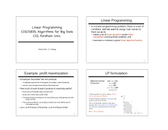
What is a linear programme? • Optimization problem consisting in • maximizing (or minimizing) a linear objective function • of n decision variables • subject to a set of constraints expressed by linear equations or inequalities. • Originally, military context: "programme"="resource planning". Now "programme"="problem" • Terminology due to George B. Dantzig, inventor of the Simplex Algorithm (1947) F . Giroire LP - Introduction 4/28

Terminology x 1 , x 2 : Decision variables 350 x 1 + 300 x 2 max Objective function subject to x 1 + x 2 ≤ 200 Constraints 9 x 1 + 6 x 2 ≤ 1566 12 x 1 + 16 x 2 ≤ 2880 x 1 , x 2 ≥ 0 F . Giroire LP - Introduction 5/28

Terminology x 1 , x 2 : Decision variables 350 x 1 + 300 x 2 max Objective function subject to x 1 + x 2 ≤ 200 Constraints 9 x 1 + 6 x 2 ≤ 1566 12 x 1 + 16 x 2 ≤ 2880 x 1 , x 2 ≥ 0 In linear programme: objective function + constraints are all linear Typically (not always): variables are non-negative If variables are integer: system called Integer Programme (IP) F . Giroire LP - Introduction 6/28

Terminology Linear programmes can be written under the standard form: ∑ n Maximize j = 1 c j x j ∑ n Subject to: ≤ for all 1 ≤ i ≤ m (1) j = 1 a ij x j b i x j ≥ 0 for all 1 ≤ j ≤ n . • the problem is a maximization; • all constraints are inequalities (and not equations); • all variables are non-negative. F . Giroire LP - Introduction 7/28

Example 1: a resource allocation problem A company produces copper cable of 5 and 10 mm of diameter on a single production line with the following constraints: • The available copper allows to produces 21000 meters of cable of 5 mm diameter per week. • A meter of 10 mm diameter copper consumes 4 times more copper than a meter of 5 mm diameter copper. Due to demand, the weekly production of 5 mm cable is limited to 15000 meters and the production of 10 mm cable should not exceed 40% of the total production. Cable are respectively sold 50 and 200 euros the meter. What should the company produce in order to maximize its weekly revenue? F . Giroire LP - Introduction 8/28

Example 1: a resource allocation problem A company produces copper cable of 5 and 10 mm of diameter on a single production line with the following constraints: • The available copper allows to produces 21000 meters of cable of 5 mm diameter per week. • A meter of 10 mm diameter copper consumes 4 times more copper than a meter of 5 mm diameter copper. Due to demand, the weekly production of 5 mm cable is limited to 15000 meters and the production of 10 mm cable should not exceed 40% of the total production. Cable are respectively sold 50 and 200 euros the meter. What should the company produce in order to maximize its weekly revenue? F . Giroire LP - Introduction 8/28

Example 1: a resource allocation problem Define two decision variables: • x 1 : the number of thousands of meters of 5 mm cables produced every week • x 2 : the number of thousands meters of 10 mm cables produced every week The revenue associated to a production ( x 1 , x 2 ) is z = 50 x 1 + 200 x 2 . The capacity of production cannot be exceeded x 1 + 4 x 2 ≤ 21 . F . Giroire LP - Introduction 9/28

Example 1: a resource allocation problem The demand constraints have to be satisfied x 2 ≤ 4 10 ( x 1 + x 2 ) x 1 ≤ 15 Negative quantities cannot be produced x 1 ≥ 0 , x 2 ≥ 0 . F . Giroire LP - Introduction 10/28

Example 1: a resource allocation problem The model: To maximize the sell revenue, determine the solutions of the following linear programme x 1 and x 2 : z = 50 x 1 + 20 x 2 max subject to x 1 + 4 x 2 ≤ 21 − 4 x 1 + 6 x 2 ≤ 0 x 1 ≤ 15 x 1 , x 2 ≥ 0 F . Giroire LP - Introduction 11/28

Example 2: Scheduling • m = 3 machines • n = 8 tasks • Each task lasts x units of time Objective: affect the tasks to the machines in order to minimize the duration • Here, the 8 tasks are finished after 7 units of times on 3 machines. F . Giroire LP - Introduction 12/28

Example 2: Scheduling • m = 3 machines • n = 8 tasks • Each task lasts x units of time Objective: affect the tasks to the machines in order to minimize the duration • Now, the 8 tasks are accomplished after 6.5 units of time: OPT? • m n possibilities! (Here 3 8 = 6561) F . Giroire LP - Introduction 12/28

Example 2: Scheduling • m = 3 machines • n = 8 tasks • Each task lasts x units of time Solution: LP model. min t subject to ∑ 1 ≤ i ≤ n t i x j i ≤ t ( ∀ j , 1 ≤ j ≤ m ) ∑ 1 ≤ j ≤ m x j i = 1 ( ∀ i , 1 ≤ i ≤ n ) with x j i = 1 if task i is affected to machine j . F . Giroire LP - Introduction 12/28

Solving Difficult Problems • Difficulty: Large number of solutions. • Choose the best solution among 2 n or n ! possibilities: all solutions cannot be enumerated. • Complexity of studied problems: often NP-complete. • Solving methods: • Optimal solutions: • Graphical method (2 variables only). • Simplex method. • Approximations: • Theory of duality (assert the quality of a solution). • Approximation algorithms. F . Giroire LP - Introduction 13/28

Graphical Method • The constraints of a linear programme define a zone of solutions. • The best point of the zone corresponds to the optimal solution. • For problem with 2 variables, easy to draw the zone of solutions and to find the optimal solution graphically. F . Giroire LP - Introduction 14/28

Graphical Method Example: 350 x 1 + 300 x 2 max subject to x 1 + x 2 ≤ 200 9 x 1 + 6 x 2 ≤ 1566 12 x 1 + 16 x 2 ≤ 2880 x 1 , x 2 ≥ 0 F . Giroire LP - Introduction 15/28

Graphical Method F . Giroire LP - Introduction 16/28

Graphical Method F . Giroire LP - Introduction 17/28

Graphical Method F . Giroire LP - Introduction 18/28

Graphical Method F . Giroire LP - Introduction 19/28

Graphical Method F . Giroire LP - Introduction 20/28

Graphical Method F . Giroire LP - Introduction 21/28

Computation of the optimal solution The optimal solution is at the intersection of the constraints: x 1 + x 2 = 200 (2) 9 x 1 + 6 x 2 = 1566 (3) We get: x 1 = 122 x 2 = 78 Objective = 66100 . F . Giroire LP - Introduction 22/28

Optimal Solutions: Different Cases F . Giroire LP - Introduction 23/28

Optimal Solutions: Different Cases Three different possible cases: • a single optimal solution, • an infinite number of optimal solutions, or • no optimal solutions. F . Giroire LP - Introduction 23/28

Optimal Solutions: Different Cases Three different possible cases: • a single optimal solution, • an infinite number of optimal solutions, or • no optimal solutions. If an optimal solution exists, there is always a corner point optimal solution! F . Giroire LP - Introduction 23/28

Solving Linear Programmes F . Giroire LP - Introduction 24/28

Solving Linear Programmes • The constraints of an LP give rise to a geometrical shape: a polyhedron. • If we can determine all the corner points of the polyhedron, then we calculate the objective function at these points and take the best one as our optimal solution. • The Simplex Method intelligently moves from corner to corner until it can prove that it has found the optimal solution. F . Giroire LP - Introduction 25/28

Solving Linear Programmes • Geometric method impossible in higher dimensions • Algebraical methods: • Simplex method (George B. Dantzig 1949): skim through the feasible solution polytope. Similar to a "Gaussian elimination". Very good in practice, but can take an exponential time. • Polynomial methods exist: • Leonid Khachiyan 1979: ellipsoid method. But more theoretical than practical. • Narendra Karmarkar 1984: a new interior method. Can be used in practice. F . Giroire LP - Introduction 26/28

But Integer Programming (IP) is different! • Feasible region: a set of discrete points. • Corner point solution not assured. • No "efficient" way to solve an IP . • Solving it as an LP provides a relaxation and a bound on the solution. F . Giroire LP - Introduction 27/28

Summary: To be remembered • What is a linear programme. • The graphical method of resolution. • Linear programs can be solved efficiently (polynomial). • Integer programs are a lot harder (in general no polynomial algorithms). In this case, we look for approximate solutions. F . Giroire LP - Introduction 28/28