Lecture #5: Multiple Linear Regression Data Science 1 CS 109A, STAT - PowerPoint PPT Presentation

Lecture #5: Multiple Linear Regression Data Science 1 CS 109A, STAT 121A, AC 209A, E-109A Pavlos Protopapas Kevin Rader Margo Levine Rahul Dave

Lecture Outline Review More on Model Evaluation Multiple Linear Regression Evaluating Significance of Predictors Comparison of Two Models Multiple Regression with Interaction Terms Polynomial Regression 2

Review 3

Statistical Models We will assume that the response variable, Y , relates to the predictors, X , through some unknown function expressed generally as: Y = f ( X ) + ϵ, where ϵ is a random variable representing measurement noise. A statistical model is any algorithm that estimates the function f . We denote the estimated function as � f and the predicted value of Y given X = x i as � y i . When performing inference , we compute parameters of � f that minimizes the error of our model, where error is measured by a choice of loss function . 4

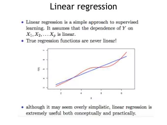
Simple Linear Regression A simple linear regression model assume that our statistical model is Y = f ( X ) + ϵ = β true X + β true + ϵ, 1 0 then it follows that � f must look like f ( X ) = � � β 1 X + � β 0 . When fitting our model, we find � β 0 , � β 1 to minimize the loss function, for example, β 0 , � � β 1 = argmin L ( β 0 , β 1 ) . β 0 ,β 1 The line � Y = � β 1 X + � β 0 is called the regression line . 5

More on Model Evaluation 6

Loss Functions Revisited Recall that there are multiple ways to measure the fitness of a model, i.e. there are multiple loss functions . 1. ( Max absolute deviation ) Count only the biggest ‘error’ max | y i − � y i | i 2. ( Sum of absolute deviations ) Add up the ‘errors’ ∑ ∑ 1 or | y i − � y i | | y i − � y i | n i i 3. ( Sum of squared errors ) Add up the squared ‘errors’ ∑ ∑ 1 y i | 2 or y i | 2 | y i − � | y i − � n i i The average squared error is the Mean Squared Error . 7

Model Fitness: R 2 While loss functions measure the predictive errors made by a model, we are also interested in the ability of our models to capture interesting features or variations in the data. We compute the explained variance or R 2 , the ratio of the variation of the model and the variation in the data. The explained variance of a regression line is given by ∑ n i =1 | y i − y i | 2 R 2 = 1 − ∑ n y i − y i | 2 i =1 | ˆ For a regression line, we have that 0 ≤ R 2 ≤ 1 Can you see why? 8

Model Evaluation: Standard Errors Rather than evaluating the predictive powers of our model or the explained variance, we can evaluate how confident we are in our estimates, � β 0 , � β 1 , of the model parameters. Recall that our estimates � β 0 , � β 1 will vary depending on the observed data. Thus, the variance of � β 0 , � β 1 indicates the extend to which we can rely on any given estimate of these parameters. The variance of � β 0 , � β 1 are also called their standard errors . 9

Model Evaluation: Standard Errors If our data is drawn from a larger set of observations then we can empirically estimate the standard errors of β 0 , � � β 1 through bootstrapping. If we know the variance σ 2 of the noise ϵ , we can ( ) ( ) � � compute SE analytically, using the β 0 , SE β 1 formulae we derived in the last lecture for � β 0 , � β 1 : √ ( ) x 2 1 � SE β 0 = σ n + ∑ i ( x i − x ) 2 ( ) σ � = √∑ SE β 1 i ( x i − x ) 2 9

Model Evaluation: Standard Errors In practice, we do not know the theoretical value of σ 2 , since we do not know the exact distribution of the noise ϵ . However, if we make the following assumptions, ▶ the errors ϵ i = y i − � y i and ϵ j = y j − � y j are uncorrelated, for i ̸ = j , ▶ each ϵ i is normally distributed with mean 0 and variance σ 2 , then, we can empirically estimate σ 2 from the data and our regression line: √∑ √ y i ) 2 n · MSE i ( y i − � σ ≈ = . n − 2 n − 2 9

Model Evaluation: Confidence Intervals Definition A n % confidence interval of an estimate � X is the range of values such that the true value of X is contained in this interval with n percent probability. For linear regression, the 95% confidence interval for β 0 , � � β 1 can be approximated using their standard errors: ( ) β k = � � � β k ± 2 SE β k for k = 0 , 1 . Thus, with approximately 95% probability, the true value of � β k is contained in the interval [ ( ) ( )] � � , � � . β k − 2 SE β k + 2 SE β k β k 10

Model Evaluation: Residual Analysis When we estimated the variance of ϵ , we assumed that the residuals ϵ i = y i − � y i were uncorrelated and normally distributed with mean 0 and fixed variance. These assumptions need to be verified using the data. In residual analysis, we typically create two types of plots: 1. a plot of ϵ i with respect to x i . This allows us to compare the distribution of the noise at different values of x i . 2. a histogram of ϵ i . This allows us to explore the distribution of the noise independent of x i . 11

A Simple Example 12

Multiple Linear Regression 13

Multilinear Models In practice, it is unlikely that any response variable Y depends solely on one predictor x . Rather, we expect that Y is a function of multiple predictors f ( X 1 , . . . , X J ) . In this case, we can still assume a simple form for f - a multilinear form: y = f ( X 1 , . . . , X J ) + ϵ = β 0 + β 1 x 1 + . . . + β J x J + ϵ. Hence, � f has the form y = � f ( X 1 , . . . , X J ) = � β 0 + � β 1 x 1 + . . . + � � β J x J . Again, to fit this model means to compute � β 0 , . . . , � β J to minimize a loss function; we will again choose the MSE as our loss function. 14

Multiple Linear Regression Given a set of observations { ( x 1 , 1 , . . . , x 1 ,J , y 1 ) , . . . ( x n, 1 , . . . , x n,J , y n ) } , the data and the model can be expressed in vector notation,       1 x 1 , 1 . . . x 1 ,J β 0 y 1     1 x 2 , 1 . . . x 2 ,J β 1 .       . Y = X = . . . β = β .  .  ,  ...  ,  β   ,  . . . .  . . .  . y y 1 x n, 1 . . . x n,J β J Thus, the MSE can be expressed in vector notation as β ) = 1 MSE ( β n ∥ Y − Xβ ∥ 2 . β Minimizing the MSE using vector calculus yields, ( ) − 1 � X ⊤ X X ⊤ Y = argmin MSE ( β β = β β β β ) . β β β 15

A Simple Example 16

Evaluating Significance of Predictors 17

Finding Significant Predictors: Hypothesis Testing With multiple predictors, an obvious analysis is to check which predictor or group of predictors have a ‘significant’ impact on the response variable. One way to do this is to analyze the ‘likelihood’ that any one or any set of regression coefficient is zero. Significant predictors will have coefficients that are deemed less ‘likely’ to be zero. Unfortunately, since the regression coefficient vary depending on the data, we cannot simply pick out non-zero coefficients from our estimate β β . β 18

Finding Significant Predictors: Hypothesis Testing Hypothesis Testing Hypothesis testing is a formal process through which we evaluate the validity of a statistical hypothesis by considering evidence for or against the hypothesis gathered by random sampling of the data. 1. State the hypotheses, typically a null hypothesis , H 0 , and an alternative hypothesis , H 1 , that is the negation of the former. 2. Choose a type of analysis, i.e. how to use sample data to evaluate the null hypothesis. Typically this involves choosing a single test statistic. 3. Sample data and compute the test statistic. 4. Use the value of the test statistic to either reject or not reject the null hypothesis. 18

Finding Significant Predictors: Hypothesis Testing For checking the significance of linear regression coefficients: 1. We set up our hypotheses (Null) H 0 : β 0 = β 1 = . . . = β J = 0 H 1 : β j ̸ = 0 , for at least one j (Alternative) 2. we choose the F -stat to evaluate the null hypothesis, explained variance F = unexplained variance 3. we can compute the F -stat for linear regression models by ∑ ∑ F = ( TSS − RSS )/ J TSS = ( y i − y ) , RSS = ( y i − � y i ) RSS /( n − J − 1) , i i 4. If F = 1 we consider this evidence for H 0 ; if F > 1 , we consider this evidence against H 0 . 18

More on Hypothesis Testing Applying the F -stat test to { X 1 , . . . , X J } determines if any of the predictors have a significant relationship with the response. We can also apply the test to a subset of predictors to determine if a smaller group of predictors have a significant relationship with the response. Note: There is not a fixed threshold for rejecting the null hypothesis based on the F -stat. For n and J that are large, F values that are slightly above 1 are considered to be strong evidence against H 0 . 19