Lecture 2: Single processor architecture and memory David Bindel - PowerPoint PPT Presentation

Lecture 2: Single processor architecture and memory David Bindel 27 Jan 2010

Logistics ◮ If we’re still overcrowded today, will request different room. ◮ Hope to have cluster account information on Monday.

The idealized machine ◮ Address space of named words ◮ Basic operations are register read/write, logic, arithmetic ◮ Everything runs in the program order ◮ High-level language translates into “obvious” machine code ◮ All operations take about the same amount of time

The real world ◮ Memory operations are not all the same! ◮ Registers and caches lead to variable access speeds ◮ Different memory layouts dramatically affect performance ◮ Instructions are non-obvious! ◮ Pipelining allows instructions to overlap ◮ Different functional units can run in parallel (and out of order) ◮ Instructions take different amounts of time ◮ Different costs for different orders and instruction mixes Our goal: enough understanding to help the compiler out.

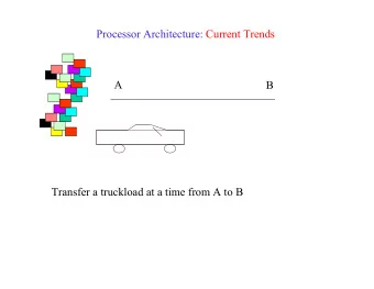
Pipelining ◮ Patterson’s example: laundry folding ◮ Pipelining improves bandwidth , but not latency ◮ Potential speedup = number of stages

Example: My laptop 2.5 GHz MacBook Pro with Intel Core 2 Duo T9300 processor. ◮ 14 stage pipeline (note: P4 was 31, but longer isn’t always better) ◮ Wide dynamic execution: up to four full instructions at once ◮ Operations internally broken down into “micro-ops” ◮ Cache micro-ops – like a hardware JIT?! In principle, two cores can handle twenty billion ops per second?

SIMD ◮ S ingle I nstruction M ultiple D ata ◮ Old idea had a resurgence in mid-late 90s (for graphics) ◮ Now short vectors are ubiquitous...

My laptop ◮ SSE (Streaming SIMD Extensions) ◮ Operates on 128 bits of data at once 1. Two 64-bit floating point or integer ops 2. Four 32-bit floating point or integer ops 3. Eight 16-bit integer ops 4. Sixteen 8-bit ops ◮ Floating point handled slightly differently from “main” FPU ◮ Requires care with data alignment Also have vector processing on GPU

Punchline ◮ Lots of special features: SIMD instructions, maybe FMAs, ... ◮ Compiler understands how to utilize these in principle ◮ Rearranges instructions to get a good mix ◮ Tries to make use of FMAs, SIMD instructions, etc ◮ In practice, needs some help: ◮ Set optimization flags, pragmas, etc ◮ Rearrange code to make things obvious ◮ Use special intrinsics or library routines ◮ Choose data layouts, algorithms that suit the machine

Cache basics Programs usually have locality ◮ Spatial locality : things close to each other tend to be accessed consecutively ◮ Temporal locality : use a “working set” of data repeatedly Cache hierarchy built to use locality.

Cache basics ◮ Memory latency = how long to get a requested item ◮ Memory bandwidth = how fast memory can provide data ◮ Bandwidth improving faster than latency Caches help: ◮ Hide memory costs by reusing data ◮ Exploit temporal locality ◮ Use bandwidth to fetch a cache line all at once ◮ Exploit spatial locality ◮ Use bandwidth to support multiple outstanding reads ◮ Overlap computation and communication with memory ◮ Prefetching This is mostly automatic and implicit.

Teaser We have N = 10 6 two-dimensional coordinates, and want their centroid. Which of these is faster and why? 1. Store an array of ( x i , y i ) coordinates. Loop i and simultaneously sum the x i and the y i . 2. Store an array of ( x i , y i ) coordinates. Loop i and sum the x i , then sum the y i in a separate loop. 3. Store the x i in one array, the y i in a second array. Sum the x i , then sum the y i . Let’s see!

Cache basics ◮ Store cache line s of several bytes ◮ Cache hit when copy of needed data in cache ◮ Cache miss otherwise. Three basic types: ◮ Compulsory miss: never used this data before ◮ Capacity miss: filled the cache with other things since this was last used – working set too big ◮ Conflict miss: insufficient associativity for access pattern ◮ Associativity ◮ Direct-mapped: each address can only go in one cache location (e.g. store address xxxx1101 only at cache location 1101) ◮ n -way: each address can go into one of n possible cache locations (store up to 16 words with addresses xxxx1101 at cache location 1101). Higher associativity is more expensive.

Caches on my laptop (I think) ◮ 32K L1 data and memory caches (per core) ◮ 8-way set associative ◮ 64-byte cache line ◮ 6 MB L2 cache (shared by both cores) ◮ 16-way set associative ◮ 64-byte cache line

A memory benchmark (membench) for array A of length L from 4 KB to 8MB by 2x for stride s from 4 bytes to L/2 by 2x time the following loop for i = 0 to L by s load A[i] from memory

membench on my laptop 60 4KB 8KB 16KB 32KB 50 64KB 128KB 256KB 512KB 40 1MB 2MB 4MB Time (nsec) 8MB 16MB 30 32MB 64MB 20 10 0 4 16 64 256 1K 4K 16K 64K 256K 1M 2M 4M 8M 16M 32M Stride (bytes)

Visible features ◮ Line length at 64 bytes (prefetching?) ◮ L1 latency around 4 ns, 8 way associative ◮ L2 latency around 14 ns ◮ L2 cache size between 4 MB and 8 MB (actually 6 MB) ◮ 4K pages, 256 entries in TLB

The moral Even for simple programs, performance is a complicated function of architecture! ◮ Need to understand at least a little in order to write fast programs ◮ Would like simple models to help understand efficiency ◮ Would like common tricks to help design fast codes ◮ Example: blocking (also called tiling )

Matrix multiply Consider naive square matrix multiplication: #define A(i,j) AA[j*n+i] #define B(i,j) BB[j*n+i] #define C(i,j) CC[j*n+i] for (i = 0; i < n; ++i) { for (j = 0; j < n; ++j) { C(i,j) = 0; for (k = 0; k < n; ++k) C(i,j) += A(i,k)*B(k,j); } } How fast can this run?

Note on storage Two standard matrix layouts: ◮ Column-major (Fortran): A(i,j) at A+j*n+i ◮ Row-major (C): A(i,j) at A+i*n+j I default to column major. Also note: C doesn’t really support matrix storage.

1000-by-1000 matrix multiply on my laptop ◮ Theoretical peak: 10 Gflop/s using both cores ◮ Naive code: 330 MFlops (3.3% peak) ◮ Vendor library: 7 Gflop/s (70% peak) Tuned code is 20 × faster than naive! Can we understand naive performance in terms of membench?

1000-by-1000 matrix multiply on my laptop ◮ Matrix sizes: about 8 MB. ◮ Repeatedly scans B in memory order (column major) ◮ 2 flops/element read from B ◮ 3 ns/flop = 6 ns/element read from B ◮ Check membench — gives right order of magnitude!

Simple model Consider two types of memory (fast and slow) over which we have complete control. ◮ m = words read from slow memory ◮ t m = slow memory op time ◮ f = number of flops ◮ t f = time per flop ◮ q = f / m = average flops / slow memory access Time: � 1 + t m / t f � ft f + mt m = ft f q Larger q means better time.

How big can q be? 1. Dot product: n data, 2 n flops 2. Matrix-vector multiply: n 2 data, 2 n 2 flops 3. Matrix-matrix multiply: 2 n 2 data, 2 n 2 flops These are examples of level 1, 2, and 3 routines in Basic Linear Algebra Subroutines (BLAS). We like building things on level 3 BLAS routines.