Hidden Markov Models George Konidaris gdk@cs.brown.edu Fall 2019 - PowerPoint PPT Presentation

Hidden Markov Models George Konidaris gdk@cs.brown.edu Fall 2019

Recall: Bayesian Network Flu Allergy Sinus Nose Headache

Recall: BN Flu Allergy Flu P Allergy P True 0.6 True 0.2 Sinus False 0.4 False 0.8 Sinus Flu Allergy P True True True 0.9 False True True 0.1 Headache True True False 0.6 False True False 0.4 True False False 0.2 False False False 0.8 Nose True False True 0.4 False False True 0.6 Headache Sinus P Nose Sinus P True True 0.6 False True 0.4 True True 0.8 True False 0.5 False True 0.2 False False 0.5 True False 0.3 joint: 32 (31) entries False False 0.7

Inference Given A compute P(B | A). Flu Allergy Sinus Nose Headache

Time Bayesian Networks (so far) contain no notion of time . However, in many applications: • Target tracking • Patient monitoring • Speech recognition • Gesture recognition … how a signal changes over time is critical.

States In probability theory, we talked about atomic events: • All possible outcomes. • Mutually exclusive. In time series, we have state : • System is in a state at time t. • Describes system completely. • Over time, transition from state to state .

Example The weather today can be: • Hot • Cold • Chilly • Freezing The weather has four states . At each point in time , the system is in one (and only one) state .

Example t=1 t=2 t=3 t=n … Freezing Freezing Freezing Freezing Chilly Chilly Chilly Chilly Hot Hot Hot Hot State transition State at time t

The Markov Assumption We are probabilistic modelers, so we’d like to model: P ( S t | S t − 1 , S t − 2 , ..., S 0 ) A state has the Markov property when we can write this as: P ( S t | S t − 1 ) Special kind of independence assumption: • Future independent of past given present.

Markov Assumption Model that has it is a Markov model . Sequence of states thus generated is a Markov chain . Definition of a state: • Sufficient statistic for history • P ( S t | S t − 1 , ..., S 0 ) = P ( S t | S t − 1 ) Can describe transition probabilities with matrix: • P(S i | S j ) • Steady state probabilities. • Convergence rates.

State Machines 0.4 A B 0.8 0.6 0.2 states not 0.5 0.5 state vars! P(A | B) = 0.8 C P(A | C) = 0.5 P(B | A) = 0.4 A B C P(B | C) = 0.5 A 0.0 0.8 0.5 P(C | A) = 0.6 B 0.4 0.0 0.5 P(C | B) = 0.2 C 0.6 0.2 0.0 Time implicit

State Machines Assumptions: • Markov assumption. • Transition probabilities don’t change with time. • Event space doesn’t change with time. • Time moves in discrete increments.

Hidden State State machines are cool but: • Often state is not observed directly. • State is latent, or hidden. State: forehand Instead you see an observation , which contains information about the hidden state.

Examples State Observation Word Phoneme Chemical State Color, Smell, etc. Flu? Runny Nose Cardiac Arrest? Pulse Sensor

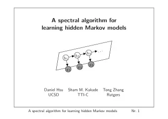
Hidden Markov Models transition model S t S t+1 observation model Must store: • P(O | S) • P(S t+1 | S t ) O t+1 O t

HMMs Monitoring/Filtering P(S t | O 0 … O t ) • E.g., estimate patient disease state. • Prediction P(S t | O 0 … O k ), k < t. • Given first two phonemes, what word? • Smoothing P(S t | O 0 … O k ), k > t • What happened back there? • Most Likely Path P(S 0 … S t | O 0 … O t ) • • How did I get here?

Example: Robot Localization observations: states: walls each side? position

Example: Robot Localization We start off not knowing where the robot is.

Example: Robot Localization Robot sense: obstacles up and down. Updates distribution.

Example: Robot Localization Robot moves right: updates distribution.

Example: Robot Localization Obstacles up and down, updates distribution.

What Happened This is an instance of robot tracking - filtering . Could also: • Predict (where will the robot be in 3 steps?) • Smooth (where was the robot?) • Most likely path (what was the robot’s path?) All of these are questions about the HMM’s state at various times.

How? S t S t+1 O t+1 O t Let’s look at P(S t ) - no observations. Assume we have CPTs

Prediction S 2 S 0 S 1 a a a b b b P(S 1 = a) = P(S 0 = a)P(a | a) + P(S 0 ) P(S 0 = b)P(a | b) (prior) P(S 1 = b) = P(S 0 = a)P(b | a) + P(S 0 = b)P(b | b)

Prediction S 2 S 0 S 1 a a a b b b P(S 2 = a) = P(S 1 = a)P(a | a) + P(S 0 ) P(S 1 ) P(S 1 = b)P(a | b) (prior) P(S 2 = b) = P(S 1 = a)P(b | a) + P(S 1 = b)P(b | b)

Filtering S t S t+1 O t+1 O t Max P(S t | O 0 … O t ). S t

Filtering Where to start? P(S t | O 0 … O t )? Let’s use P(S t, O 0 … O t ). X P ( S t , O 0 , ..., O t ) = P ( S t , S t − 1 = s i , O 0 , ..., O t ) i X = P ( O t | S t ) P ( S t | S t − 1 = s i ) P ( S t − 1 = s i , O 0 , ..., O t − 1 ) i X = P ( O t | S t ) P ( S t | S t − 1 = s i ) P ( S t − 1 = s i , O 0 , ..., O t − 1 ) i

Forward Algorithm Let F(k, 0) = P(S 0 = s k )P(O 0 | S 0 = s k ) . For t = 1, …, T: For k in possible states: X F ( k, t ) = P ( O t | S t = s k ) P ( s k | s i ) F ( i, t − 1) i F(k, T) is P(S T = s k , O 0 … O T ) (normalize to get P(S T | O 0 … O T ))

Smoothing P(S t | O 0 … O k ), k > t - given data of length k, find P(S t ) for earlier t . Bayes Rule: • P(S t | O 0 … O k ) P(O 0 … O k | S t ) P(S t | O 0 … O k ) ∝ • P(O t … O k | S t ) P(S t | O 0 … O t ) ∝ forward algorithm forward algorithm Compute using backward pass: P(O i … O k | S i ) computed using similar recursion. Forward-backward algorithm.

Most Likely Path S t S t+1 O t+1 O t max P(S 0 … S t | O 0 … O t ) S 0 … S t

Viterbi Similar logic to highest probability state, but: • We seek a path , not a state . • Single highest probability state. • Therefore look for highest probability of (ancestor probability times observation probability) • Maintain link matrix to read path backwards Similar dynamic programming algorithm, replace sum with max .

Viterbi Algorithm Most likely path S 0 … S n : V i,k : probability of max prob. path at ending in state s k, including observations up to O i (t=i). L i,k : most likely predecessor of state s k at time i . For each state s k : observation V 0,k = P(O 0 | s k )P(s k ) transition model model L 0,k = 0 For i = 1…n , probability For each k : of path to x V i,k = P(O i | s k ) max x P(s k | s x ) V i-1 , x L i,k = argmax x P(s k | s x )V i-1,x most likely ancestor

Common Form Very common form: • Noisy observations of true state

Viterbi “The algorithm has found universal application in decoding the convolutional codes used in both CDMA and GSM digital cellular, dial-up modems, satellite, deep-space communications, and 802.11 wireless LANs.” (wikipedia) (photo credit: MIT)