Gov 2000: 8. Simple Linear Regression Matthew Blackwell Fall 2016 - PowerPoint PPT Presentation
Gov 2000: 8. Simple Linear Regression Matthew Blackwell Fall 2016 1 / 84 1. Assumptions of the Linear Regression Model 2. Sampling Distribution of the OLS Estimator 3. Sampling Variance of the OLS Estimator 4. Large Sample Properties of OLS
Gov 2000: 8. Simple Linear Regression Matthew Blackwell Fall 2016 1 / 84
1. Assumptions of the Linear Regression Model 2. Sampling Distribution of the OLS Estimator 3. Sampling Variance of the OLS Estimator 4. Large Sample Properties of OLS 5. Exact Inference for OLS 6. Hypothesis Tests and Confjdence Intervals 7. Goodness of Fit 2 / 84
Where are we? Where are we going? intervals 3 / 84 • Last week: ▶ Using the CEF to explore relationships ▶ Practical estimation concerns led us to OLS/lines of best fjt. • This week: ▶ Inference for OLS: sampling distribution. ▶ Is there really a relationship? Hypothesis tests ▶ Can we get a range of plausible slope values? Confjdence ▶ ⇝ how to read regression output.
More narrow goal ## ## logem4 -0.5641 0.0639 -8.83 2.1e-13 *** ## --- ## Signif. codes: 0 '***' 0.001 '**' 0.01 '*' 0.05 '.' 0.1 ' ' 1 ## Residual standard error: 0.756 on 79 degrees of freedom 34.92 ## (82 observations deleted due to missingness) ## Multiple R-squared: 0.497, Adjusted R-squared: 0.49 ## F-statistic: 78 on 1 and 79 DF, p-value: 2.09e-13 < 2e-16 *** 0.3053 ## 3Q ## Call: ## lm(formula = logpgp95 ~ logem4, data = ajr) ## ## Residuals: ## Min 1Q Median Max 10.6602 ## -2.7130 -0.5333 0.0195 0.4719 1.4467 ## ## Coefficients: ## Estimate Std. Error t value Pr(>|t|) ## (Intercept) 4 / 84
1/ Assumptions of the Linear Regression Model 5 / 84
Simple linear regression model than 𝑌 𝑗 . 6 / 84 • We are going to assume a linear model: 𝑍 𝑗 = 𝛾 0 + 𝛾 1 𝑌 𝑗 + 𝑣 𝑗 • Data: ▶ Dependent variable: 𝑍 𝑗 ▶ Independent variable: 𝑌 𝑗 • Population parameters: ▶ Population intercept: 𝛾 0 ▶ Population slope: 𝛾 1 • Error/disturbance: 𝑣 𝑗 ▶ Represents all unobserved error factors infmuencing 𝑍 𝑗 other
Causality and regression regression we called the linear projection. causal or structural. factors ( 𝑣 𝑗 ) constant. 7 / 84 𝑍 𝑗 = 𝛾 0 + 𝛾 1 𝑌 𝑗 + 𝑣 𝑗 • Last week we showed there is always a population linear ▶ No notion of causality and may not even be the CEF. • Traditional regression approach: assume slope parameters are ▶ 𝛾 1 is the efgect of a one-unit change in 𝑦 holding all other • Regression will always consistently estimate a linear association between 𝑍 𝑗 and 𝑌 𝑗 . • Today: When will regression say something causal? ▶ GOV 2001/2002 has more on a formal language of causality.
Linear regression model need to make some statistical assumptions: Linear Regression Model The observations, (𝑍 𝑗 , 𝑌 𝑗 ) come from a random (i.i.d.) sample and satisfy the linear regression equation, 𝔽[𝑣 𝑗 |𝑌 𝑗 ] = 0. The independent variable is assumed to have non-zero variance, 𝕎[𝑌 𝑗 ] > 0 . 8 / 84 • In order to investigate the statistical properties of OLS, we 𝑍 𝑗 = 𝛾 0 + 𝛾 1 𝑌 𝑗 + 𝑣 𝑗
Linearity Assumption 1: Linearity The population regression function is linear in the parameters: 1 + 𝑣 𝑗 non-linearities in 𝑌 𝑗 . 9 / 84 𝑍 𝑗 = 𝛾 0 + 𝛾 1 𝑌 𝑗 + 𝑣 𝑗 • Violation of the linearity assumption: 𝑍 𝑗 = 𝛾 0 + 𝛾 1 𝑌 𝑗 • Not a violation of the linearity assumption: 𝑍 𝑗 = 𝛾 0 + 𝛾 1 𝑌 2 𝑗 + 𝑣 𝑗 • In future weeks, we’ll talk about how to allow for
Random sample Assumption 2: Random Sample We have a iid random sample of size 𝑜 , {(𝑍 𝑗 , 𝑌 𝑗 ) ∶ 𝑗 = 1, 2, … , 𝑜} from the population regression model above. minutes the day before: 10 / 84 • Violations: time-series, selected samples. • Think about the weight example from last week, where 𝑍 𝑗 was my weight on a given day and 𝑌 𝑗 was my number of active weight 𝑗 = 𝛾 0 + 𝛾 1 activity 𝑗 + 𝑣 𝑗 • What if I only weighed myself on the weekdays?
A non-iid sample 11 / 84 0 -1 Y -2 -3 0 20 40 60 80 100 X
Variation in X Assumption 3: Variation in 𝑌 There is in-sample variation in 𝑌 𝑗 , so that, 𝑜 ∑ 𝑗=1 ̂ ∑ 𝑜 12 / 84 (𝑌 𝑗 − 𝑌) 2 > 0. • OLS not well-defjned if no in-sample variation in 𝑌 𝑗 • Remember the formula for the OLS slope estimator: 𝛾 1 = ∑ 𝑜 𝑗=1 (𝑌 𝑗 − 𝑌)(𝑍 𝑗 − 𝑍) 𝑗=1 (𝑌 𝑗 − 𝑌) 2 • What happens here when 𝑌 𝑗 doesn’t vary?
Stuck in a moment assumption? 13 / 84 fjt through this scatterplot, which is a violation of this • Why does this matter? How would you draw the line of best 2 1 0 Y -1 -2 -3 -2 -1 0 1 2 3 X
Stuck in a moment assumption? 14 / 84 fjt through this scatterplot, which is a violation of this • Why does this matter? How would you draw the line of best 2 1 0 Y -1 -2 -3 -2 -1 0 1 2 3 X
Zero conditional mean Assumption 4: Zero conditional mean of the errors The error, 𝑣 𝑗 , has expected value of 0 given any value of the independent variable: ∀𝑦. Cov [𝑣 𝑗 , 𝑌 𝑗 ] = 𝔽[𝑣 𝑗 𝑌 𝑗 ] = 0 15 / 84 𝔽[𝑣 𝑗 |𝑌 𝑗 = 𝑦] = 0 • ⇝ weaker condition that 𝑣 𝑗 and 𝑌 𝑗 uncorrelated: • ⇝ 𝔽[𝑍 𝑗 |𝑌 𝑗 ] = 𝛾 0 + 𝛾 1 𝑌 𝑗 is the CEF
Violating the zero conditional 2. No relationship between them (satisfjes the assumption) mean assumption 16 / 84 from the following model: • How does this assumption get violated? Let’s generate data 𝑍 𝑗 = 1 + 0.5𝑌 𝑗 + 𝑣 𝑗 • But let’s compare two situations: 1. Where the mean of 𝑣 𝑗 depends on 𝑌 𝑗 (they are correlated) Assumption 4 violated Assumption 4 not violated 5 5 4 4 3 3 2 2 Y Y 1 1 0 0 -1 -1 -2 -2 -3 -2 -1 0 1 2 3 -3 -2 -1 0 1 2 3 X X
More examples of zero conditional mean in the error minutes the day before: etc. mean, no matter what my level of activity was. Plausible? assigned. 17 / 84 • Think about the weight example from last week, where 𝑍 𝑗 was my weight on a given day and 𝑌 𝑗 was my number of active weight 𝑗 = 𝛾 0 + 𝛾 1 activity 𝑗 + 𝑣 𝑗 • What might in 𝑣 𝑗 here? Amount of food eaten, workload, etc • We have to assume that all of these factors have the same • When is this assumption most plausible? When 𝑌 𝑗 is randomly
2/ Sampling Distribution of the OLS Estimator 18 / 84
What is OLS? 𝑜 ∑ 𝑜 ̂ 𝛾 1 𝑌 ̂ ∑ 𝑗=1 𝑐 0 ,𝑐 1 𝛾 1 ) = arg min residuals: the intercept of the regression line. 19 / 84 • Ordinary least squares (OLS) is an estimator for the slope and • Where does it come from? Minimizing the sum of the squared ( ̂ 𝛾 0 , ̂ (𝑍 𝑗 − 𝑐 0 − 𝑐 1 𝑌 𝑗 ) 2 • Leads to: 𝛾 0 = 𝑍 − ̂ 𝛾 1 = ∑ 𝑜 𝑗=1 (𝑌 𝑗 − 𝑌)(𝑍 𝑗 − 𝑍) 𝑗=1 (𝑌 𝑗 − 𝑌) 2
Intuition of the OLS estimator = Sample Variance of 𝑌 𝕎[𝑌 𝑗 ] ̂ Cov (𝑌 𝑗 , 𝑍 𝑗 ) ̂ ∑ 𝑜 𝛾 1 𝑌 ̂ 20 / 84 • Regression line goes through the sample means (𝑍, 𝑌) : 𝑍 = ̂ 𝛾 0 + ̂ • Slope is the ratio of the covariance to the variance of 𝑌 𝑗 : 𝛾 1 = ∑ 𝑜 𝑗=1 (𝑌 𝑗 − 𝑌)(𝑍 𝑗 − 𝑍) 𝑗=1 (𝑌 𝑗 − 𝑌) 2 = Sample Covariance between 𝑌 and 𝑍
The sample linear regression 𝛾 0 estimates. 𝑍 𝑗 ̂ 𝑍 𝑗 function 𝛾 1 ̂ 𝛾 1 𝑌 𝑗 21 / 84 • The estimated or sample regression function is: 𝑍 𝑗 = ̂ 𝛾 0 + ̂ • Estimated intercept: ̂ • Estimated slope: ̂ • Predicted/fjtted values: ̂ 𝑣 𝑗 = 𝑍 𝑗 − ̂ • Residuals: • You can think of the residuals as the prediction errors of our
OLS slope as a weighted sum of the outcomes 𝑋 𝑗 𝑣 𝑗 𝑗=1 ∑ 𝑜 ̂ proof ∑ 𝑜 22 / 84 𝑋 𝑗 𝑍 𝑗 ̂ 𝑗=1 ∑ the OLS estimator for the slope as a weighted sum of the outcomes. 𝑜 • One useful derivation that we’ll do moving forward is to write 𝛾 1 = • Where here we have the weights, 𝑋 𝑗 as: (𝑌 𝑗 − 𝑌) 𝑋 𝑗 = 𝑗=1 (𝑌 𝑗 − 𝑌) 2 • Estimation error: 𝛾 1 − 𝛾 1 = • ⇝ ̂ 𝛾 1 is a sum of random variables.
Sampling distribution of the OLS ⋮ variance/standard error, etc. sample variance 𝛾 1 ) 𝑙 (̂ Sample 𝑙 : {(𝑍 1 , 𝑌 1 ), … , (𝑍 𝑜 , 𝑌 𝑜 )} 𝛾 1 ) 𝑙−1 (̂ Sample 𝑙 − 1 : {(𝑍 1 , 𝑌 1 ), … , (𝑍 𝑜 , 𝑌 𝑜 )} estimator ⋮ 𝛾 1 ) 2 (̂ Sample 2: {(𝑍 1 , 𝑌 1 ), … , (𝑍 𝑜 , 𝑌 𝑜 )} 𝛾 1 ) 1 (̂ Sample 1: {(𝑍 1 , 𝑌 1 ), … , (𝑍 𝑜 , 𝑌 𝑜 )} OLS data into and we get out estimates. 23 / 84 • Remember: OLS is an estimator—it’s a machine that we plug 𝛾 0 , ̂ 𝛾 0 , ̂ 𝛾 0 , ̂ 𝛾 0 , ̂ • Just like the sample mean, sample difgerence in means, or the • It has a sampling distribution, with a sampling
Simulation procedure interest 1. Draw a random sample of size 𝑜 = 30 with replacement using sample() 2. Use lm() to calculate the OLS estimates of the slope and intercept 3. Plot the estimated regression line 24 / 84 • Let’s take a simulation approach to demonstrate: ▶ Pretend that the AJR data represents the population of ▶ See how the line varies from sample to sample
Population Regression 25 / 84 12 11 Log GDP per capita 10 9 8 7 6 1 2 3 4 5 6 7 8 Log Settler Mortality
Recommend
More recommend
Explore More Topics
Stay informed with curated content and fresh updates.
