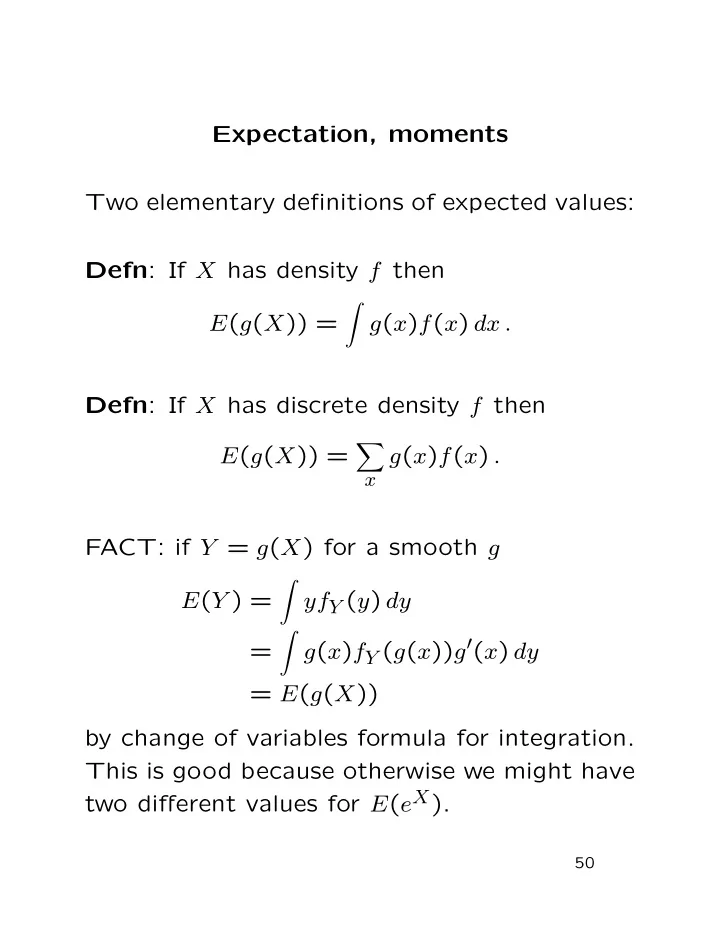
Expectation, moments Two elementary definitions of expected values: - PDF document

Expectation, moments Two elementary definitions of expected values: Defn : If X has density f then � E ( g ( X )) = g ( x ) f ( x ) dx . Defn : If X has discrete density f then � E ( g ( X )) = g ( x ) f ( x ) . x FACT: if Y = g ( X ) for a smooth g � E ( Y ) = yf Y ( y ) dy � g ( x ) f Y ( g ( x )) g ′ ( x ) dy = = E ( g ( X )) by change of variables formula for integration. This is good because otherwise we might have two different values for E ( e X ). 50

Defn : X is integrable if E ( | X | ) < ∞ . Facts: E is a linear, monotone, positive oper- ator: 1. Linear : E ( aX + bY ) = aE ( X )+ bE ( Y ) pro- vided X and Y are integrable. 2. Positive : P ( X ≥ 0) = 1 implies E ( X ) ≥ 0. 3. Monotone : P ( X ≥ Y ) = 1 and X , Y inte- grable implies E ( X ) ≥ E ( Y ). 51

Defn : The r th moment (about the origin) of r = E ( X r ) (provided it exists). a real rv X is µ ′ We generally use µ for E ( X ). Defn : The r th central moment is µ r = E [( X − µ ) r ] We call σ 2 = µ 2 the variance. Defn : For an R p valued random vector X µ X = E ( X ) is the vector whose i th entry is E ( X i ) (provided all entries exist). Defn : The ( p × p ) variance covariance matrix of X is � ( X − µ )( X − µ ) t � Var( X ) = E which exists provided each component X i has a finite second moment. 52

Moments and probabilities of rare events are closely connected as will be seen in a number of important probability theorems. Example : Markov’s inequality P ( | X − µ | ≥ t ) = E [1( | X − µ | ≥ t )] | X − µ | r � � ≤ E 1( | X − µ | ≥ t ) t r ≤ E [ | X − µ | r ] t r Intuition: if moments are small then large de- viations from average are unlikely. Special case is Chebyshev’s inequality: P ( | X − µ | ≥ t ) ≤ Var( X ) . t 2 53

Example moments : If Z ∼ N (0 , 1) then � ∞ √ −∞ ze − z 2 / 2 dz/ E ( Z ) = 2 π ∞ � = − e − z 2 / 2 � √ � � 2 π � � −∞ = 0 and (integrating by parts) � ∞ √ −∞ z r e − z 2 / 2 dz/ E ( Z r ) = 2 π ∞ � = − z r − 1 e − z 2 / 2 � √ � � 2 π � � −∞ � ∞ √ −∞ z r − 2 e − z 2 / 2 dz/ + ( r − 1) 2 π so that µ r = ( r − 1) µ r − 2 for r ≥ 2. Remembering that µ 1 = 0 and � ∞ √ −∞ z 0 e − z 2 / 2 dz/ µ 0 = 2 π = 1 we find that � 0 r odd µ r = ( r − 1)( r − 3) · · · 1 r even . 54

If now X ∼ N ( µ, σ 2 ), that is, X ∼ σZ + µ , then E ( X ) = σE ( Z ) + µ = µ and µ r ( X ) = E [( X − µ ) r ] = σ r E ( Z r ) In particular, we see that our choice of nota- tion N ( µ, σ 2 ) for the distribution of σZ + µ is justified; σ is indeed the variance. Similarly for X ∼ MV N ( µ, Σ) we have X = AZ + µ with Z ∼ MV N (0 , I ) and E ( X ) = µ and � ( X − µ )( X − µ ) t � Var( X ) = E � AZ ( AZ ) t � = E = AE ( ZZ t ) A t = AIA t = Σ . Note use of easy calculation: E ( Z ) = 0 and Var( Z ) = E ( ZZ t ) = I . 55