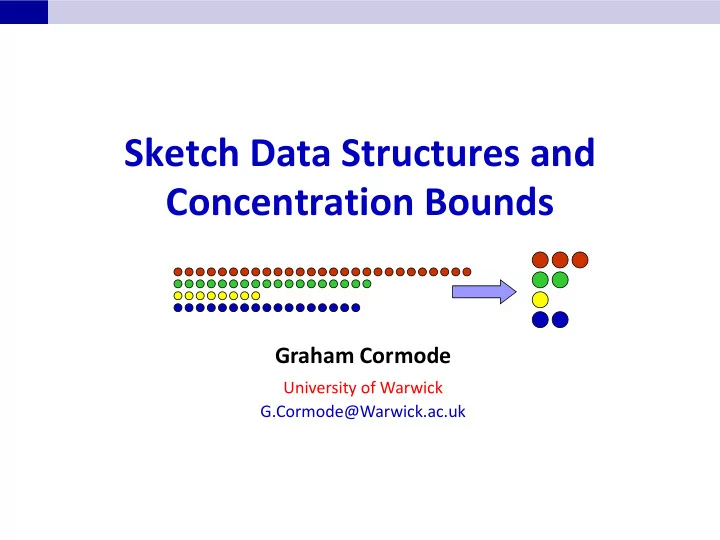
Sketch Data Structures and Concentration Bounds Graham Cormode - PowerPoint PPT Presentation

Sketch Data Structures and Concentration Bounds Graham Cormode University of Warwick G.Cormode@Warwick.ac.uk

Big Data  “Big” data arises in many forms: – Physical Measurements: from science (physics, astronomy) – Medical data: genetic sequences, detailed time series – Activity data: GPS location, social network activity – Business data: customer behavior tracking at fine detail  Common themes: – Data is large, and growing – There are important patterns and trends in the data – We don’t fully know how to find them 2 Small Summaries for Big Data

Making sense of Big Data  Want to be able to interrogate data in different use-cases: – Routine Reporting: standard set of queries to run – Analysis : ad hoc querying to answer ‘data science’ questions – Monitoring: identify when current behavior differs from old – Mining: extract new knowledge and patterns from data  In all cases, need to answer certain basic questions quickly: – Describe the distribution of particular attributes in the data – How many (distinct) X were seen? – How many X < Y were seen? – Give some representative examples of items in the data 3 Small Summaries for Big Data

Data Models  We model data as a collection of simple tuples  Problems hard due to scale and dimension of input  Arrivals only model: x – Example: (x, 3), (y, 2), (x, 2) encodes the arrival of 3 copies of item x, y 2 copies of y, then 2 copies of x. – Could represent eg. packets on a network; power usage  Arrivals and departures: x – Example: (x, 3), (y,2), (x, -2) encodes y final state of (x, 1), (y, 2). – Can represent fluctuating quantities, or measure differences between two distributions 4 Sketch Data Structures and Concentration Bounds

Sketches and Frequency Moments  Frequency distributions and Concentration bounds  Count-Min sketch for F  and frequent items  AMS Sketch for F 2  Estimating F 0  Extensions: – Higher frequency moments – Combined frequency moments 5 Sketch Data Structures and Concentration Bounds

Frequency Distributions  Given set of items, let f i be the number of occurrences of item i  Many natural questions on f i values: – Find those i ’s with large f i values (heavy hitters) – Find the number of non-zero f i values (count distinct) – Compute F k =  i (f i ) k – the k ’th Frequency Moment – Compute H =  i (f i /F 1 ) log (F 1 /f i ) – the (empirical) entropy  “ Space Complexity of the Frequency Moments ” Alon, Matias, Szegedy in STOC 1996 – Awarded Gödel prize in 2005 – Set the pattern for many streaming algorithms to follow 6 Sketch Data Structures and Concentration Bounds

Concentration Bounds  Will provide randomized algorithms for these problems  Each algorithm gives a (randomized) estimate of the answer  Give confidence bounds on the final estimate X – Use probabilistic concentration bounds on random variables  A concentration bound is typically of the form Pr[ |X – x| >  y ] <  – At most probability  of being more than  y away from x Probability distribution Tail probability  7 Sketch Data Structures and Concentration Bounds

Markov Inequality  Take any probability distribution X s.t. Pr[X < 0] = 0  Consider the event X  k for some constant k > 0  For any draw of X, k I (X  k)  X k |X| – Either 0  X < k, so I (X  k) = 0 – Or X  k, lhs = k  Take expectations of both sides: k Pr[ X  k]  E[X]  Markov inequality: Pr[ X  k ]  E[X]/k – Prob of random variable exceeding k times its expectation < 1/k – Relatively weak in this form, but still useful 8 Sketch Data Structures and Concentration Bounds

Sketch Structures  Sketch is a class of summary that is a linear transform of input – Sketch(x) = Sx for some matrix S – Hence, Sketch(  x +  y) =  Sketch(x) +  Sketch(y) – Trivial to update and merge  Often describe S in terms of hash functions – If hash functions are simple, sketch is fast  Aim for limited independence hash functions h: [n]  [m] – If Pr h  H [ h(i 1 )=j 1  h(i 2 )=j 2  … h(i k )=j k ] = m -k , then H is k- wise independent family (“ h is k- wise independent”) – k-wise independent hash functions take time, space O(k) 9 Sketch Data Structures and Concentration Bounds

Sketches and Frequency Moments  Frequency distributions and Concentration bounds  Count-Min sketch for F  and frequent items  AMS Sketch for F 2  Estimating F 0  Extensions: – Higher frequency moments – Combined frequency moments 10 Sketch Data Structures and Concentration Bounds

Count-Min Sketch  Simple sketch idea relies primarily on Markov inequality  Model input data as a vector x of dimension U  Creates a small summary as an array of w  d in size  Use d hash function to map vector entries to [1..w]  Works on arrivals only and arrivals & departures streams W Array: d CM[i,j] 11 Sketch Data Structures and Concentration Bounds

Count-Min Sketch Structure +c h 1 (j) d=log 1/  +c j,+c +c h d (j) +c w = 2/   Each entry in vector x is mapped to one bucket per row.  Merge two sketches by entry-wise summation  Estimate x[j] by taking min k CM[k,h k (j)] – Guarantees error less than  F 1 in size O(1/  log 1/  ) – Probability of more error is less than 1-  [C, Muthukrishnan ’04] 12 Sketch Data Structures and Concentration Bounds

Approximation of Point Queries Approximate point query x’[j] = min k CM[k,h k (j)]  Analysis: In k'th row, CM[k,h k (j)] = x[j] + X k,j – X k,j = S i x[i] I (h k (i) = h k (j)) = S i  j x[i]*Pr[h k (i)=h k (j)] – E[X k,j ]  Pr[h k (i)=h k (j)] * S i x[i] =  F 1 /2 – requires only pairwise independence of h – Pr[X k,j   F 1 ] = Pr[ X k,j  2E[X k,j ] ]  1/2 by Markov inequality  So, Pr[x’[j]  x[j] +  F 1 ] = Pr[  k. X k,j >  F 1 ]  1/2 log 1/  =   Final result: with certainty x[j]  x’[j] and with probability at least 1-  , x’[j] < x[j] +  F 1 13 Sketch Data Structures and Concentration Bounds

Applications of Count-Min to Heavy Hitters  Count-Min sketch lets us estimate f i for any i (up to  F 1 )  Heavy Hitters asks to find i such that f i is large (>  F 1 )  Slow way: test every i after creating sketch  Alternate way: – Keep binary tree over input domain: each node is a subset – Keep sketches of all nodes at same level – Descend tree to find large frequencies, discard ‘light’ branches – Same structure estimates arbitrary range sums  A first step towards compressed sensing style results... 14 Sketch Data Structures and Concentration Bounds

Application to Large Scale Machine Learning  In machine learning, often have very large feature space – Many objects, each with huge, sparse feature vectors – Slow and costly to work in the full feature space  “ Hash kernels ”: work with a sketch of the features – Effective in practice! [Weinberger, Dasgupta, Langford, Smola, Attenberg ‘09]  Similar analysis explains why: – Essentially, not too much noise on the important features 15 Sketch Data Structures and Concentration Bounds

Sketches and Frequency Moments  Frequency distributions and Concentration bounds  Count-Min sketch for F  and frequent items  AMS Sketch for F 2  Estimating F 0  Extensions: – Higher frequency moments – Combined frequency moments 16 Sketch Data Structures and Concentration Bounds

Chebyshev Inequality  Markov inequality is often quite weak  But Markov inequality holds for any random variable  Can apply to a random variable that is a function of X  Set Y = (X – E[X]) 2  By Markov, Pr[ Y > kE[Y] ] < 1/k – E[Y] = E[(X-E[X]) 2 ]= Var[X]  Hence, Pr[ |X – E[X]| > √(k Var[X]) ] < 1/k  Chebyshev inequality: Pr[ |X – E[X]| > k ] < Var[X]/k 2 – If Var[X]   2 E[X] 2 , then Pr[|X – E[X]| >  E[X] ] = O(1) 17 Sketch Data Structures and Concentration Bounds

F 2 estimation  AMS sketch (for Alon-Matias-Szegedy) proposed in 1996 – Allows estimation of F 2 (second frequency moment) – Used at the heart of many streaming and non-streaming applications: achieves dimensionality reduction  Here, describe AMS sketch by generalizing CM sketch.  Uses extra hash functions g 1 ...g log 1/  {1...U}  {+1,-1} – (Low independence) Rademacher variables  Now, given update (j,+c), set CM[k,h k (j)] += c*g k (j) linear projection AMS sketch 18 Sketch Data Structures and Concentration Bounds

F 2 analysis +c*g 1 (j) h 1 (j) d=8log 1/  +c*g 2 (j) j,+c +c*g 3 (j) h d (j) +c*g 4 (j) w = 4 /  2  Estimate F 2 = median k  i CM[k,i] 2  Each row’s result is  i g(i) 2 x[i] 2 +  h(i)=h(j) 2 g(i) g(j) x[i] x[j]  But g(i) 2 = -1 2 = +1 2 = 1, and  i x[i] 2 = F 2  g(i)g(j) has 1/2 chance of +1 or –1 : expectation is 0 … 19 Sketch Data Structures and Concentration Bounds