Randomized Algorithms Balls-into-bins model The threshold for - PowerPoint PPT Presentation
Randomized Algorithms Balls-into-bins model The threshold for throw m balls into n bins being 1-1 is uniformly and independently m = ( n ). uniform random function The threshold for f : [ m ] [ n ]
Randomized Algorithms 南京大学 尹一通
Balls-into-bins model • The threshold for throw m balls into n bins being 1-1 is uniformly and independently m = Θ ( √ n ). uniform random function • The threshold for f : [ m ] → [ n ] being on-to is m = n ln n + O ( n ). 1-1 birthday problem • The maximum load is on-to coupon collector � O ( ln n ln ln n ) for m = Θ ( n ) , O ( m n ) for m = Ω ( n ln n ) . pre-images occupancy problem
Stable Marriage n men n women • each man has a preference order of the n women; • each woman has a preference order of the n men; • solution: n couples • Marriage is stable!
Stable Marriage n men n women unstable: exist a man and women, who prefer each other to their prefer current partners prefer stability: local optimum fixed point equilibrium deadlock
Proposal Algorithm (Gale-Shapley 1962) Single man: propose p propose to the most r o p o s e propose preferable women who has not rejected him Woman: upon received a proposal : accept if she’s single or married to a less preferable man ( divorce! ) n men n women
Proposal Algorithm Single man: • woman: once got married always married propose to the most (will only switch to better men!) preferable women who • man: will only get worse ... has not rejected him • once all women are married, the algorithm Woman: terminates, and the upon received a proposal : marriages are stable accept if she’s single or • total number of proposals: married to a less preferable man ≤ n 2 ( divorce! )
Average-case women change men propose minds • every man/woman has a uniform random permutation as preference list • total number of proposals? everyone has an ordered list. proposing, rejected, accepted, running off with another man ... Looks very complicated!
Principle of Deferred Decisions Principle of deferred decision The decision of random choice in the random input is deferred to the running time of the algorithm.
Principle of Deferred Decisions women change proposing in the men propose minds order of a uniformly random permutation at each time, proposing to a uniformly random woman who has not rejected him decisions of the inputs are deferred to the time when Alg accesses them
Principle of Deferred Decisions women change at each time, proposing to men propose minds a uniformly random woman who has not rejected him ≤ uniform & independent at each time, proposing to a uniformly & independently random woman the man forgot who had rejected him (!)
Principle of Deferred Decisions • uniformly and independently proposing to n women • Alg stops once all women got proposed. uniform & independent • Coupon collector! • Expected O( n ln n ) proposals.
Tail Inequalities
Pretty: Tail bound : Pr[ X > t ] < � . Good Thresholding: � • The running time of a Las Ugly: Vegas Alg. • Some cost (e.g. max load). • The probability of extreme case. Good �
n-ball-to-n-bin: Tail bound : Pr[load of the first bin ≥ t ] Pr[ X > t ] < � . �⇧ 1 ⌥ ⌃ t n ≤ t n Take I: Counting n ! = t !( n − t )! n t • calculation = 1 t ! · n ( n − 1)( n − 2) ··· ( n − t + 1) • smartness n t t − 1 = 1 ⇧ ⌃ 1 − i ⇥ t ! · n i = 0 tail bounds for dummies? ≤ 1 t ! ⇤ e ⌅ t ≤ t
Tail bound : X follows distribution Pr[ X > t ] < � . D Take II: Characterizing Relate tail to some measurable characters of X character I Reduce the tail bound to the analysis of the characters. Pr[ X > t ] < f ( t , I )
Markov’s Inequality Markov’s Inequality: For nonnegative X , for any t > 0, Pr[ X ≥ t ] ≤ E [ X ] . t Proof : � X � 1 if X ≥ t , ⇥ ≤ X Let Y = ⇒ Y ≤ t , t 0 otherwise. � X ⇥ = E [ X ] Pr[ X ≥ t ] = E [ Y ] ≤ E . t t QED tight if we only know the expectation of X
Las Vegas to Monte Carlo • Las Vegas: running time is B(x): random, always correct. run A(x) for 2T(n) steps; if A(x) returned • A : Las Vegas Alg with return A(x); worst-case expected else return 1 ; running time T ( n ) . one-sided error! • Monte Carlo: running Pr[error] time is fixed, correct with chance. ≤ Pr[ T ( A ( x )) > 2 T ( n )] • B : Monte Carlo Alg ... ≤ 1 ≤ E [ T ( A ( x ))] 2 T ( n ) 2 ZPP ⊆ RP
A Generalization of Markov’s Inequality Theorem: For any X , for h : X ⇥� R + , for any t > 0, Pr[ h ( X ) ≥ t ] ≤ E [ h ( X )] . t Chebyshev, Chernoff, ...
Chebyshev’s Inequality Chebyshev’s Inequality: For any t > 0, Pr[ | X − E [ X ] | ≥ t ] ≤ Var [ X ] . t 2
Variance Definition ( variance ) : The variance of a random variable X is ( X − E [ X ]) 2 ⇥ X 2 ⇥ − ( E [ X ]) 2 . � � Var [ X ] = E = E The standard deviation of random variable X is � δ [ X ] = Var [ X ]
Covariance Definition ( covariance ) : The covariance of X and Y is Cov ( X , Y ) = E [( X − E [ X ])( Y − E [ Y ])]. Theorem: Var [ X + Y ] = Var [ X ] + Var [ Y ] + 2 Cov ( X , Y ); � ⇥ n n ⇤ ⇤ ⇤ Var X i Var [ X i ] + Cov ( X i , X j ). = i = 1 i = 1 i � = j
Covariance Theorem: For independent X and Y , E [ X · Y ] = E [ X ] · E [ Y ]. Theorem: For independent X and Y , Cov ( X , Y ) = 0. Proof : Cov ( X , Y ) = E [( X − E [ X ])( Y − E [ Y ])] = E [ X − E [ X ]] E [ Y − E [ Y ]] = 0.
Variance of sum Theorem: For independent X and Y , Cov ( X , Y ) = 0. Theorem: For pairwise independent X 1 , X 2 ,..., X n , � ⇥ n n ⇤ ⇤ X i Var [ X i ]. Var = i = 1 i = 1
Variance of Binomial Distribution • Binomial distribution: number of successes in n i.i.d. Bernoulli trials. • X follows binomial distribution with parameter n and p � n 1 with probability p � X = X i X i = 0 with probability 1 − p i = 1 Var [ X i ] = E [ X 2 i ] − E [ X i ] 2 = p − p 2 = p (1 − p ) n � (independence) Var [ X ] = Var [ X i ] = p (1 − p ) n i = 1
Chebyshev’s Inequality Chebyshev’s Inequality: For any t > 0, Pr[ | X − E [ X ] | ≥ t ] ≤ Var [ X ] . t 2 Proof : Apply Markov’s inequality to ( X − E [ X ]) 2 ( X − E [ X ]) 2 ⇥ � E ( X − E [ X ]) 2 ≥ t 2 ⇥ � Pr ≤ t 2 QED
Selection Problem Input: a set of n elements Output: median straightforward alg: sorting, Ω ( n log n ) time sophisticated deterministic alg: median of medians, Θ ( n ) time simple randomized alg: LazySelect, Θ ( n ) time, find the median whp
Selection by Sampling distribution: Naive sampling: uniformly choose an random element make a wish it is the median
Selection by Sampling distribution: R : sample a small set R , selection in R by sorting roughly concentrated, but not good enough
Selection by Sampling distributions: d u d u � C Find such d and u that: • Let C = { x ∈ S | d ≤ x ≤ u }. • The median is in C. • C is not too large (sort C is linear time).
LazySelect (Floyd & Rivest) d u R: d u Size of R : r Offset for d and u from the median of R : k Bad events: median is not between d and u ; too many elements between d and u . (inefficient to sort)
O( r log r ) 1. Uniformly and independently sample r elements from S to form R ; and sort R . O(1) 2. Let d be the ( r 2 − k )th element in R . O(1) 3. Let u be the ( r 2 + k )th element in R . O( n ) 4. If any of the following occurs | { x ∈ S | x < d } | > n 2 ; | { x ∈ S | x > u } | > n 2 ; | { x ∈ S | d ≤ x ≤ u } | > s ; Pr[FAIL] < ? then FAIL. O( s log s ) 5. Find the median of S by sorting { x ∈ S | d ≤ x ≤ u }.
Bad events: 1. | { x ∈ S | x < d } | > n 2 ; 2. | { x ∈ S | x > u } | > n 2 ; or | { x ∈ S | x < d } | < n 2 − s 2 ; 3. | { x ∈ S | d ≤ x ≤ u } | > s ; | { x ∈ S | x > u } | < n 2 − s 2 ; s Symmetry! � S : d u Bad events for d : d is too large: R : d u | { x ∈ S | x < d } | > n 2 � r samples d is too small: k offset | { x ∈ S | x < d } | < n 2 − s 2
Bad events for d : Bad events for R : d is too large: the sample of rank r 2 − k | { x ∈ S | x < d } | > n is ranked > n 2 in S . 2 d is too small: the sample of rank r 2 − k | { x ∈ S | x < d } | < n 2 − s is ranked ≤ n 2 − s 2 in S . 2 s � S : d u R : d u R : r uniform and � independent samples from S r samples k offset
Bad events for d : Bad events for R : d is too large: < r 2 − k samples are among | { x ∈ S | x < d } | > n the smallest half in S . 2 d is too small: � r 2 � k samples are among | { x ∈ S | x < d } | < n 2 − s the n 2 � s 2 smallest in S . 2 s � S : d u R : d u R : r uniform and � independent samples from S r samples k offset
i th sample R : r uniform and 1 ranks ≤ n /2, independent samples from S X i = otherwise. 0 Bad events for R : r � X = X i < r 2 − k samples are among E 1 : i = 1 the smallest half in S . i th sample 1 ≥ r ranks ≤ n 2 − s E 2 : 2 − k samples are among 2 , Y i = the n 2 − s 2 smallest in S . otherwise. 0 r n 2 − s � Y = Y i 2 � i = 1 S: � n r samples 2
Recommend
More recommend
Explore More Topics
Stay informed with curated content and fresh updates.
