Randomized Algorithms, Quicksort and Randomized Selection Carola - PowerPoint PPT Presentation
CMPS 2200 Fall 2014 Randomized Algorithms, Quicksort and Randomized Selection Carola Wenk Slides courtesy of Charles Leiserson with additions by Carola Wenk CMPS 2200 Intro. to Algorithms 1 Deterministic Algorithms Runtime for
CMPS 2200 – Fall 2014 Randomized Algorithms, Quicksort and Randomized Selection Carola Wenk Slides courtesy of Charles Leiserson with additions by Carola Wenk CMPS 2200 Intro. to Algorithms 1
Deterministic Algorithms Runtime for deterministic algorithms with input size n : • Best-case runtime Attained by one input of size n • Worst-case runtime Attained by one input of size n • Average runtime Averaged over all possible inputs of size n CMPS 2200 Intro. to Algorithms 2
Deterministic Algorithms: Insertion Sort for j=2 to n { key = A[j] // insert A[j] into sorted sequence A[1..j-1] i=j-1 while(i>0 && A[i]>key){ A[i+1]=A[i] i-- } A[i+1]=key } • Best case runtime? • Worst case runtime? CMPS 2200 Intro. to Algorithms 3
Deterministic Algorithms: Insertion Sort Best-case runtime: O ( n ), input [1,2,3,…, n ] Attained by one input of size n • Worst-case runtime: O ( n 2 ), input [ n , n -1, …,2,1] Attained by one input of size n • Average runtime : O ( n 2 ) Averaged over all possible inputs of size n •What kind of inputs are there? • How many inputs are there? CMPS 2200 Intro. to Algorithms 4
Average Runtime • What kind of inputs are there? • Do [1,2,…, n ] and [5,6,…, n +5] cause different behavior of Insertion Sort? • No. Therefore it suffices to only consider all permutations of [1,2,…, n ] . • How many inputs are there? • There are n ! different permutations of [1,2,…, n ] CMPS 2200 Intro. to Algorithms 5
Average Runtime Insertion Sort: n =4 • Inputs: 4!=24 0 3 4 6 [1,2,3,4] [4,1,2,3] [4,1,3,2] [4,3,2,1] 1 2 3 5 [2,1,3,4] [1,4,2,3] [1,4,3,2] [3,4,2,1] 1 1 2 4 [1,3,2,4] [1,2,4,3] [1,3,4,2] [3,2,4,1] 2 4 5 5 [3,1,2,4] [4,2,1,3] [4,3,1,2] [4,2,3,1] 3 2 4 4 [3,2,1,4] [2,1,4,3] [3,4,1,2] [2,4,3,1] 2 3 3 3 [2,3,1,4] [2,4,1,3] [3,1,4,2] [2,3,4,1] • Runtime is proportional to: 3 + #times in while loop • Best: 3+ 0 , Worst: 3+ 6 =9, Average: 3+ 72 /24 = 6 CMPS 2200 Intro. to Algorithms 6
Average Runtime: Insertion Sort • The average runtime averages runtimes over all n ! different input permutations • Disadvantage of considering average runtime: • There are still worst-case inputs that will have the worst-case runtime • Are all inputs really equally likely? That depends on the application Better: Use a randomized algorithm CMPS 2200 Intro. to Algorithms 7
Randomized Algorithm: Insertion Sort • Randomize the order of the input array: • Either prior to calling insertion sort, • or during insertion sort (insert random element) • This makes the runtime depend on a probabilistic experiment (sequence of numbers obtained from random number generator; or random input permutation) Runtime is a random variable (maps sequence of random numbers to runtimes) • Expected runtime = expected value of runtime random variable CMPS 2200 Intro. to Algorithms 8
Randomized Algorithm: Insertion Sort • Runtime is independent of input order ([1,2,3,4] may have good or bad runtime, depending on sequence of random numbers) •No assumptions need to be made about input distribution • No one specific input elicits worst-case behavior • The worst case is determined only by the output of a random-number generator. When possible use expected runtimes of randomized algorithms instead of average case analysis of deterministic algorithms CMPS 2200 Intro. to Algorithms 9
Quicksort • Proposed by C.A.R. Hoare in 1962. • Divide-and-conquer algorithm. • Sorts “in place” (like insertion sort, but not like merge sort). • Very practical (with tuning). • We are going to perform an expected runtime analysis on randomized quicksort CMPS 2200 Intro. to Algorithms 10
Quicksort: Divide and conquer Quicksort an n -element array: 1. Divide: Partition the array into two subarrays around a pivot x such that elements in lower subarray x elements in upper subarray. x x x 2. Conquer: Recursively sort the two subarrays. 3. Combine: Trivial. Key: Linear-time partitioning subroutine. CMPS 2200 Intro. to Algorithms 11
Partitioning subroutine P ARTITION ( A , p , q ) A [ p . . q ] x A [ p ] pivot = A [ p ] Running time i p = O ( n ) for n for j p + 1 to q elements. do if A [ j ] x then i i + 1 exchange A [ i ] A [ j ] exchange A [ p ] A [ i ] return i x x Invariant: x ? p i j q CMPS 2200 Intro. to Algorithms 12
Example of partitioning 6 10 13 5 8 3 2 11 i j CMPS 2200 Intro. to Algorithms 13
Example of partitioning 6 10 13 5 8 3 2 11 i j CMPS 2200 Intro. to Algorithms 14
Example of partitioning 6 10 13 5 8 3 2 11 i j CMPS 2200 Intro. to Algorithms 15
Example of partitioning 6 10 13 5 8 3 2 11 6 5 13 10 8 3 2 11 i j CMPS 2200 Intro. to Algorithms 16
Example of partitioning 6 10 13 5 8 3 2 11 6 5 13 10 8 3 2 11 i j CMPS 2200 Intro. to Algorithms 17
Example of partitioning 6 10 13 5 8 3 2 11 6 5 13 10 8 3 2 11 i j CMPS 2200 Intro. to Algorithms 18
Example of partitioning 6 10 13 5 8 3 2 11 6 5 13 10 8 3 2 11 6 5 3 10 8 13 2 11 i j CMPS 2200 Intro. to Algorithms 19
Example of partitioning 6 10 13 5 8 3 2 11 6 5 13 10 8 3 2 11 6 5 3 10 8 13 2 11 i j CMPS 2200 Intro. to Algorithms 20
Example of partitioning 6 10 13 5 8 3 2 11 6 5 13 10 8 3 2 11 6 5 3 10 8 13 2 11 6 5 3 2 8 13 10 11 i j CMPS 2200 Intro. to Algorithms 21
Example of partitioning 6 10 13 5 8 3 2 11 6 5 13 10 8 3 2 11 6 5 3 10 8 13 2 11 6 5 3 2 8 13 10 11 i j CMPS 2200 Intro. to Algorithms 22
Example of partitioning 6 10 13 5 8 3 2 11 6 5 13 10 8 3 2 11 6 5 3 10 8 13 2 11 6 5 3 2 8 13 10 11 i j CMPS 2200 Intro. to Algorithms 23
Example of partitioning 6 10 13 5 8 3 2 11 6 5 13 10 8 3 2 11 6 5 3 10 8 13 2 11 6 5 3 2 8 13 10 11 2 5 3 6 8 13 10 11 i CMPS 2200 Intro. to Algorithms 24
Pseudocode for quicksort Q UICKSORT ( A , p, r ) if p < r then q P ARTITION ( A , p, r ) Q UICKSORT ( A , p, q –1) Q UICKSORT ( A , q+ 1 , r ) Initial call: Q UICKSORT ( A , 1 , n ) CMPS 2200 Intro. to Algorithms 25
Analysis of quicksort • Assume all input elements are distinct. • In practice, there are better partitioning algorithms for when duplicate input elements may exist. • Let T(n) = worst-case running time on an array of n elements. CMPS 2200 Intro. to Algorithms 26
Worst-case of quicksort • Input sorted or reverse sorted. • Partition around min or max element. • One side of partition always has no elements. T ( n ) T ( 0 ) T ( n 1 ) ( n ) ( 1 ) ( 1 ) ( ) T n n T ( n 1 ) ( n ) 2 (arithmetic series) ( n ) CMPS 2200 Intro. to Algorithms 27
Worst-case recursion tree T ( n ) = T (0) + T ( n –1) + cn CMPS 2200 Intro. to Algorithms 28
Worst-case recursion tree T ( n ) = T (0) + T ( n –1) + cn T ( n ) CMPS 2200 Intro. to Algorithms 29
Worst-case recursion tree T ( n ) = T (0) + T ( n –1) + cn cn T (0) T ( n –1) CMPS 2200 Intro. to Algorithms 30
Worst-case recursion tree T ( n ) = T (0) + T ( n –1) + cn cn T (0) c ( n –1) T (0) T ( n –2) CMPS 2200 Intro. to Algorithms 31
Worst-case recursion tree T ( n ) = T (0) + T ( n –1) + cn cn T (0) c ( n –1) T (0) c ( n –2) T (0) (1) CMPS 2200 Intro. to Algorithms 32
Worst-case recursion tree T ( n ) = T (0) + T ( n –1) + cn height cn 2 k n T (0) c ( n –1) k 1 T (0) c ( n –2) height = n T (0) T (0) CMPS 2200 Intro. to Algorithms 33
Worst-case recursion tree T ( n ) = T (0) + T ( n –1) + cn n cn 2 k n T (0) c ( n –1) k 1 T (0) c ( n –2) height = n T (0) T (0) CMPS 2200 Intro. to Algorithms 34
Worst-case recursion tree T ( n ) = T (0) + T ( n –1) + cn n cn 2 k n (1) c ( n –1) k 1 (1) c ( n –2) T ( n ) = ( n ) + ( n 2 ) height = n (1) = ( n 2 ) (1) CMPS 2200 Intro. to Algorithms 35
Best-case analysis (For intuition only!) If we’re lucky, P ARTITION splits the array evenly: T ( n ) = 2 T ( n /2) + ( n ) = ( n log n ) (same as merge sort) 1 : 9 What if the split is always ? 10 10 T ( n ) T 1 n T 9 n ( n ) 10 10 What is the solution to this recurrence? CMPS 2200 Intro. to Algorithms 36
Analysis of “almost-best” case T ( n ) CMPS 2200 Intro. to Algorithms 37
Analysis of “almost-best” case cn T 10 1 n 9 T 10 n CMPS 2200 Intro. to Algorithms 38
Analysis of “almost-best” case cn 1 cn 9 cn 10 10 T 100 1 n T 100 9 n T 100 9 n T 100 81 n CMPS 2200 Intro. to Algorithms 39
Recommend
More recommend
Explore More Topics
Stay informed with curated content and fresh updates.
