EC3062 ECONOMETRICS THE MULTIPLE REGRESSION MODEL Consider T - PowerPoint PPT Presentation

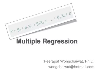
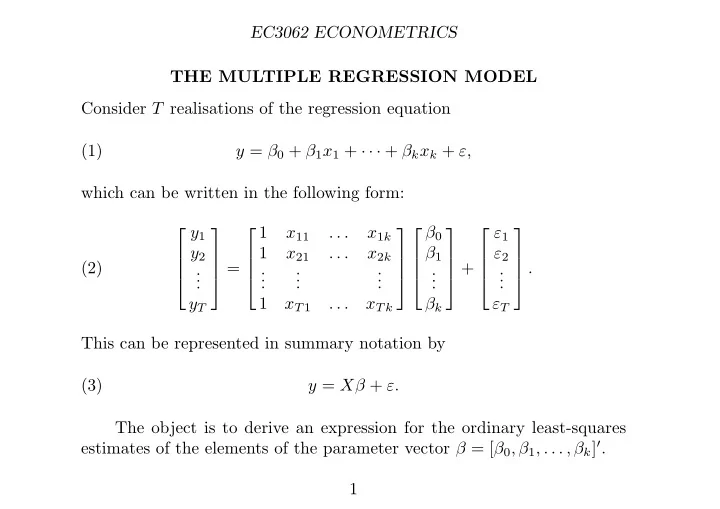
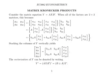
EC3062 ECONOMETRICS THE MULTIPLE REGRESSION MODEL Consider T realisations of the regression equation (1) y = β 0 + β 1 x 1 + · · · + β k x k + ε, which can be written in the following form: y 1 β 0 1 x 11 . . . x 1 k ε 1         y 2 β 1 1 x 21 . . . x 2 k ε 2         (2)  =  +  . . . . . . .         . . . . . . . . . . . .      1 x T 1 . . . x T k ε T y T β k This can be represented in summary notation by (3) y = Xβ + ε. The object is to derive an expression for the ordinary least-squares estimates of the elements of the parameter vector β = [ β 0 , β 1 , . . . , β k ] ′ . 1

EC3062 ECONOMETRICS The ordinary least-squares (OLS) estimate of β is the value that minimises S ( β ) = ε ′ ε = ( y − Xβ ) ′ ( y − Xβ ) (4) = y ′ y − y ′ Xβ − β ′ X ′ y + β ′ X ′ Xβ = y ′ y − 2 y ′ Xβ + β ′ X ′ Xβ. According to the rules of matrix differentiation, the derivative is ∂S ∂β = − 2 y ′ X + 2 β ′ X ′ X. (5) Setting this to zero gives 0 = β ′ X ′ X − y ′ X , which is transposed to provide the so-called normal equations: X ′ Xβ = X ′ y. (6) On the assumption that the inverse matrix exists, the equations have a unique solution, which is the vector of ordinary least-squares estimates: ˆ β = ( X ′ X ) − 1 X ′ y. (7) 2

EC3062 ECONOMETRICS The Decomposition of the Sum of Squares The equation y = X ˆ β + e , decomposes y into a regression component X ˆ β and a residual component e = y − ˆ Xβ . These are mutually orthogonal, since (6) indicates that X ′ ( y − ˆ Xβ ) = 0. Define the projection matrix P = X ( X ′ X ) − 1 X ′ , which is symmetric and idempotent such that P = P ′ = P 2 P ′ ( I − P ) = 0 . or, equivalently, Then, X ˆ β = Py and e = y − ˆ Xβ = ( I − P ) y , and, therefore, the regression decomposition is y = Py + ( I − P ) y. The conditions on P imply that � ′ � � � y ′ y = Py + ( I − P ) y Py + ( I − P ) y (8) = y ′ Py + y ′ ( I − P ) y = ˆ β ′ X ′ X ˆ β + e ′ e. 3

EC3062 ECONOMETRICS This is an instance of Pythagorus theorem; and the equation indicates that the total sum of squares y ′ y is equal to the regression sum of squares β ′ X ′ X ˆ ˆ β plus the residual or error sum of squares e ′ e . By projecting y perpendicularly onto the manifold of X , the distance between y and Py = X ˆ β is minimised. Proof. Let γ = Pg be an arbitrary vector in the manifold of X . Then ( y − X ˆ β ) + ( X ˆ � ′ � ( y − X ˆ β ) + ( X ˆ � � (9) ( y − γ ) ′ ( y − γ ) = β − γ ) β − γ ) � ′ � � � = ( I − P ) y + P ( y − g ) ( I − P ) y + P ( y − g ) . The properties of P indicate that ( y − γ ) ′ ( y − γ ) = y ′ ( I − P ) y + ( y − g ) ′ P ( y − g ) (10) = e ′ e + ( X ˆ β − γ ) ′ ( X ˆ β − γ ) . Since the squared distance ( X ˆ β − γ ) ′ ( X ˆ β − γ ) is nonnegative, it follows that ( y − γ ) ′ ( y − γ ) ≥ e ′ e , where e = y − X ˆ β ; which proves the assertion. 4

EC3062 ECONOMETRICS The Coefficient of Determination A summary measure of the extent to which the ordinary least-squares regression accounts for the observed vector y is provided by the coefficient of determination. This is defined by β ′ X ′ X ˆ ˆ β = y ′ Py R 2 = (11) y ′ y . y ′ y The measure is just the square of the cosine of the angle between the β ; and the inequality 0 ≤ R 2 ≤ 1 follows from the vectors y and Py = X ˆ fact that the cosine of any angle must lie between − 1 and +1. If X is a square matrix of full rank, with as many regressors as observations, then X − 1 exists and P = X ( X ′ X ) − 1 X = X { X − 1 X ′− 1 } X ′ = I, and so R 2 = 1. If X ′ y = 0, then, Py = 0 and R 2 = 0. But, if y is distibuted continuously, then this event has a zero probability. 5

EC3062 ECONOMETRICS e y ^ β X γ Figure 1. The vector Py = X ˆ β is formed by the orthogonal projec- tion of the vector y onto the subspace spanned by the columns of the matrix X . 6

EC3062 ECONOMETRICS The Partitioned Regression Model Consider partitioning the regression equation of (3) to give � � β 1 (12) y = [ X 1 X 2 ] + ε = X 1 β 1 + X 2 β 2 + ε, β 2 2 ] ′ = β . The normal equations of (6) can where [ X 1 , X 2 ] = X and [ β ′ 1 , β ′ be partitioned likewise: X ′ 1 X 1 β 1 + X ′ 1 X 2 β 2 = X ′ (13) 1 y, X ′ 2 X 1 β 1 + X ′ 2 X 2 β 2 = X ′ (14) 2 y. From (13), we get the X ′ 1 X 1 β 1 = X ′ 1 ( y − X 2 β 2 ), which gives ˆ 1 ( y − X 2 ˆ 1 X 1 ) − 1 X ′ β 1 = ( X ′ (15) β 2 ) . To obtain an expression for ˆ β 2 , we must eliminate β 1 from equation (14). 1 X 1 ) − 1 to give For this, we multiply equation (13) by X ′ 2 X 1 ( X ′ 1 X 1 ) − 1 X ′ 1 X 1 ) − 1 X ′ X ′ 2 X 1 β 1 + X ′ 2 X 1 ( X ′ 1 X 2 β 2 = X ′ 2 X 1 ( X ′ (16) 1 y. 7

EC3062 ECONOMETRICS From X ′ 2 X 1 β 1 + X ′ 2 X 2 β 2 = X ′ (14) 2 y, we take the resulting equation 1 X 1 ) − 1 X ′ 1 X 1 ) − 1 X ′ X ′ 2 X 1 β 1 + X ′ 2 X 1 ( X ′ 1 X 2 β 2 = X ′ 2 X 1 ( X ′ (16) 1 y to give � � 1 X 1 ) − 1 X ′ 1 X 1 ) − 1 X ′ X ′ 2 X 2 − X ′ 2 X 1 ( X ′ β 2 = X ′ 2 y − X ′ 2 X 1 ( X ′ (17) 1 X 2 1 y. 1 X 1 ) − 1 X ′ On defining P 1 = X 1 ( X ′ 1 , equation (17) can be written as � � X ′ β 2 = X ′ (19) 2 ( I − P 1 ) X 2 2 ( I − P 1 ) y, whence � − 1 � ˆ X ′ X ′ (20) β 2 = 2 ( I − P 1 ) X 2 2 ( I − P 1 ) y. 8

EC3062 ECONOMETRICS The Regression Model with an Intercept Consider again the equations (22) y = ια + Zβ z + ε. where ι = [1 , 1 , . . . , 1] ′ is the summation vector and Z = [ x tj ], with t = 1 , . . . T and j = 1 , . . . , k , is the matrix of the explanatory variables. This is a case of the partitioned regression equation of (12). By setting X 1 = ι and X 2 = Z and by taking β 1 = α , β 2 = β z , the equations (15) and (20), give the following estimates of the α and β z : α = ( ι ′ ι ) − 1 ι ′ ( y − Z ˆ (23) ˆ β z ) , and � − 1 Z ′ ( I − P ι ) y, ˆ � Z ′ ( I − P ι ) Z β z = with (24) P ι = ι ( ι ′ ι ) − 1 ι ′ = 1 T ιι ′ . 9

EC3062 ECONOMETRICS To understand the effect of the operator P ι , consider T T ( ι ′ ι ) − 1 ι ′ y = 1 � � ι ′ y = y t , y t = ¯ y, T (25) t =1 t =1 y = ι ( ι ′ ι ) − 1 ι ′ y = [¯ y ] ′ . and P ι y = ι ¯ y, ¯ y, . . . , ¯ y ] ′ is a column vector containing T repetitions of Here, P ι y = [¯ y, ¯ y, . . . , ¯ the sample mean. From the above, it can be understood that, if x = [ x 1 , x 2 , . . . x T ] ′ is vector of T elements, then T T T � � � x ) 2 . x ′ ( I − P ι ) x = (26) x t ( x t − ¯ x ) = ( x t − ¯ x ) x t = ( x t − ¯ t =1 t =1 t =1 The final equality depends on the fact that � ( x t − ¯ x � ( x t − ¯ x )¯ x = ¯ x ) = 0. 10

EC3062 ECONOMETRICS The Regression Model in Deviation Form Consider the matrix of cross-products in equation (24). This is Z ′ ( I − P ι ) Z = { ( I − P ι ) Z } ′ { Z ( I − P ι ) } = ( Z − ¯ Z ) ′ ( Z − ¯ (27) Z ) . Here, ¯ Z contains the sample means of the k explanatory variables repeated T times. The matrix ( I − P ι ) Z = ( Z − ¯ Z ) contains the deviations of the data points about the sample means. The vector ( I − P ι ) y = ( y − ι ¯ y ) may be described likewise. � − 1 Z ′ ( I − P ι ) y is It follows that the estimate ˆ � β z = Z ′ ( I − P ι ) Z obtained by applying the least-squares regression to the equation y 1 − ¯ y x 11 − ¯ x 1 . . . x 1 k − ¯ x k ε 1 − ¯ ε      β 1    y 2 − ¯ y x 21 − ¯ x 1 . . . x 2 k − ¯ x k ε 2 − ¯ ε .         . (28)  =  +  , . . . . .    . .     .  . . . . .      β k y T − ¯ y x T 1 − ¯ x 1 . . . x T k − ¯ x k ε T − ¯ ε which lacks an intercept term. 11

EC3062 ECONOMETRICS In summary notation, the equation may be denoted by y = [ Z − ¯ (29) y − ι ¯ Z ] β z + ( ε − ¯ ε ) . Observe that it is unnecessary to take the deviations of y . The result y on [ Z − ¯ is the same whether we regress y or y − ι ¯ Z ]. The result is due to the symmetry and idempotency of the operator ( I − P ι ), whereby Z ′ ( I − P ι ) y = { ( I − P ι ) Z } ′ { ( I − P ι ) y } . Once the value for ˆ β z is available, the estimate for the intercept term can be recovered from the equation (23), which can be written as k y − ¯ Z ˆ x j ˆ � (30) α = ¯ ˆ β z = ¯ y − ¯ β j . j =1 12