2 Y X Not linear in variables 0 1 Y X 1 Not - PDF document

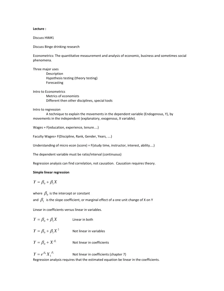
Lecture : Discuss HW#1 Discuss Binge drinking research Econometrics: The quantitative measurement and analysis of economic, business and sometimes social phenomena. Three major uses Description Hypothesis testing (theory testing) Forecasting Intro to Econometrics Metrics of economists Different then other disciplines, special tools Intro to regression A technique to explain the movements in the dependent variable (Endogenous, Y), by movements in the independent (explanatory, exogenous, X variable). Wages = F(education, experience, tenure....) Faculty Wages= F(Discipline, Rank, Gender, Years, ….) Understanding of micro econ (score) = F(study time, instructor, interest, ability....) The dependent variable must be ratio/interval (continuous) Regression analysis can find correlation, not causation. Causation requires theory. Simple linear regression     Y X 0 1  is the intercept or constant where 0  is the slope coefficient, or marginal effect of a one unit change of X on Y and 1 Linear in coefficients versus linear in variables.     Y X Linear in both 0 1     2 Y X Not linear in variables 0 1     Y X 1 Not linear in coefficients 0  X  Y  e 0 1 Not linear in coefficients (chapter 7) 1 Regression analysis requires that the estimated equation be linear in the coefficients.

The dependent variable *must* be ratio/interval (continuous) (there are some caveats)     ( ) ( ) f Y f X General form 0 1 The Stochastic Error Term There is always some variation in Y that can’t be explained. Example (performance in micro) 1. Omitted variables 2. Measurement error 3. Incorrect functional form 4. Random chance so we add a term to our equation       Y X 0 1 Two parts, deterministic, and stochastic (random)     ( | ) E Y X X 0 1 Expanded notation       i  Y X ( 1 .. n ) where and indexes individual observations 0 1 i i i so       Y X 1 0 1 1 1       Y X 2 0 1 2 2 ....       Y X 0 1 n n n REGRESSION /MISSING LISTWISE /STATISTICS COEFF OUTS R ANOVA /CRITERIA=PIN(.05) POUT(.10) /NOORIGIN /DEPENDENT salary /METHOD=ENTER market. Model Summary

Adjusted R Std. Error of the Model R R Square Square Estimate .407 a 1 .166 .164 11585.82899 a. Predictors: (Constant), market Coefficients a Standardized Unstandardized Coefficients Coefficients Model B Std. Error Beta t Sig. 3288.009 1 (Constant) 18096.994 5.504 .000 market 34545.219 3424.333 .407 10.088 .000 a. Dependent Variable: salary . r egr ess sal ar y m ar ket Sour ce SS df M S Num ber of obs = 514 514 F( 1, 512) = 101. 77 101. 77 M odel 1. 3661e+10 1 1. 3661e 1. 3661e+10 1 1. 3661e+10 +10 Pr ob > F = 0. 0000 0. 0000 Resi dual 6. 8726e+10 512 134231 6. 8726e+10 512 134231433 433 R- squar ed = 0. 1658 0. 1658 Adj R- squar ed = 0. 1642 0. 1642 Tot al 8. 2387e+10 513 160599 8. 2387e+10 513 160599133 133 Root M SE = 11586 11586 sal ar y Coef . St d. Er r . t P>| t | [ 95% Conf . I nt er val ] m ar ket 34545. 22 3424. 333 1 34545. 22 3424. 333 10. 09 0. 000 27817. 75 0. 09 0. 000 27817. 75 41272. 69 41272. 69 _cons 18096. 99 3288. 009 18096. 99 3288. 009 5. 50 0. 000 11637. 35 5. 50 0. 000 11637. 35 24556. 64 24556. 64

100000 80000 Academic salary 60000 40000 20000 .6 .8 1 1.2 1.4 salary Marketability Linear prediction

Lecture 9: Again the multivariate representation is            y x x ... x 0 1 1 2 2 i i i k ki i  ' Again the s represent the partial effects of the x Constant is a junk collector, so that the residuals sum to zero. Be careful about making inferences on the value of the constant        2       ˆ   ˆ   ˆ 2 2 ˆ y y y x x 0 1 1 2 2 i i i i i i Minimizing by differentiating with respect to the betas and solving them simultaneously yields the normal equations. http://en.wikibooks.org/wiki/Econometric_Theory/Normal_Equations_Proof (Note: There is a mistake in the derivation of the above. The solution is correct, but an n appears in front of the alpha a few equations early.) Where the solutions for the multivariate case are given here:      2 yx x yx x x  ˆ  1 2 2 1 2   1  2 2 2 x x ( x x ) 1 2 1 2      2 yx x yx x x  ˆ  2 1 1 1 2   2  2 2 2 x x ( x x ) 1 2 1 2  ˆ    ˆ   ˆ y x x 0 1 1 2 21 where the lower case letters immediately above represent deviations form their mean  i   i  x x x and x x x 1 1 1 2 2 2 Evaluating the quality of a regression. Spend time before running the regression thinking about the expected output. 1. Is the estimated equation supported by the theory? 2. How well does it fit the data? 3. Is the dataset reasonable large and accurate? 4. Is OLS the best estimator for this case? 5. How well do estimates match your prediction? 6. Any important omitted variables? 7. Has the most logical functional form been used? 8. Is the regression free from other econometric problems? Describing the fit:

Total, explained and residual sum of squares. TSS, ESS, RSS    2 ( ) TSS y y deviation of observation from mean (picture in upper left) i which can be decomposed into two parts TSS= ESS+RSS         2 2 2 ˆ ˆ ( ) ( ) ( ) y y y y y y i i i i The explained portion (ESS), from the fitted line to the mean (this is represented by the solid vertical lines in the upper right hand picture. The Residual or unexplained portion is depicted in the lowest picture. From the fitted line to the observation. 2 R (R squared) coefficient of determination 2 R = (ESS/TSS) = 1 ‐ (RSS/TSS)

 2 e  i 1   2 ( ) y y i 2   R 0 1 Be careful when comparing time series vs cross section. R squared in the .9 range is common for time series and unheard almost unheard of on cross sectional analysis. What happens when you add an explanatory variable? TSS doesn’t change, but ESS goes up. So we would always want to add a variable, but then the degrees of freedom fall. Degrees of freedom reflect the reliability of our estimates.       Y X 0 1 i i i we are estimating 2 coefficients degrees of freedom = observations ‐ 2. n ‐ 2. More generally            ... y x x x i 0 1 1 i 2 2 i k ki i we are estimating k+1 coefficients so degrees of freedom = n ‐ (k+1) we can use this information to “penalize” the inclusion of an additional variable to better reflect the tradeoff. NOTE: We cannot estimate the model if there are negative DOF. We effectively have less information than coefficients to estimate. The solution is not unique. n>k+1 is a requirement 2 R or sometimes referred to as r ‐ bar squared Adjusted       1 RSS n k   2 R 1    1 TSS n by a simple rearrangement we get        n 1    2 2   1 1 R R         1 n k note as k rises so does the penalty, whether or not it offsets the increase in R squared will impact R bar squared. Note Adjusted R squared (sometimes called R bar Squared) can be less then 0, but it is bounded above by 1. Appropriate and inappropriate uses of R bar squared COMMENT lets run our first regression. REGRESSION /MISSING LISTWISE /STATISTICS COEFF OUTS R /*I've removed the ANOVA from the default */ /CRITERIA=PIN(.05) POUT(.10) /NOORIGIN

/DEPENDENT salary /METHOD=ENTER market. Model Summary Adjusted R Std. Error of the Model R R Square Square Estimate .407 a 1 .166 .164 11585.82899 a. Predictors: (Constant), market Coefficients a Standardized Unstandardized Coefficients Coefficients Model B Std. Error Beta t Sig. 3288.009 1 (Constant) 18096.994 5.504 .000 market 34545.219 3424.333 .407 10.088 .000 a. Dependent Variable: salary COMMENT lets run our second regression adding yearsdg. REGRESSION /MISSING LISTWISE /STATISTICS COEFF OUTS R /*I've removed the ANOVA from the default */ /CRITERIA=PIN(.05) POUT(.10) /NOORIGIN /DEPENDENT salary /METHOD=ENTER market yearsdg. Model Summary Adjusted R Std. Error of the Model R R Square Square Estimate .824 a 1 .680 .678 7187.88271 a. Predictors: (Constant), yearsdg, market Coefficients a Standardized Model Unstandardized Coefficients Coefficients t Sig.

B Std. Error Beta 2153.797 1 (Constant) -1685.118 -.782 .434 market 39630.458 2131.883 .467 18.589 .000 yearsdg 979.458 34.221 .719 28.622 .000 a. Dependent Variable: salary