EC3062 ECONOMETRICS LINEAR STOCHASTIC MODELS Let { x +1 , x +2 , . - PowerPoint PPT Presentation

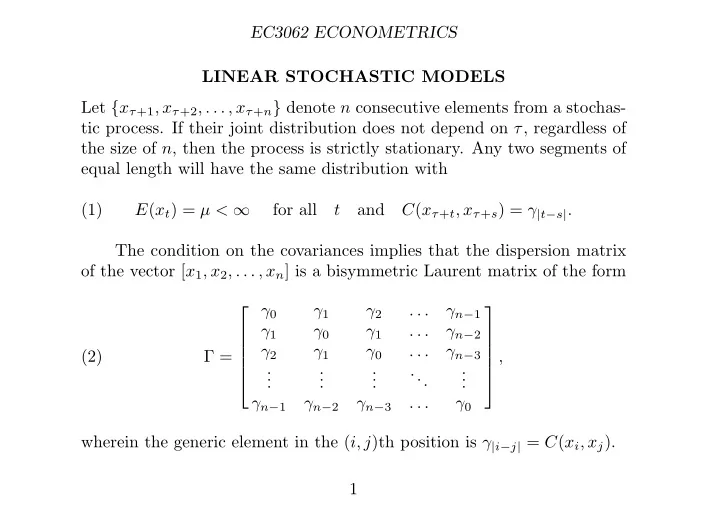
EC3062 ECONOMETRICS LINEAR STOCHASTIC MODELS Let { x τ +1 , x τ +2 , . . . , x τ + n } denote n consecutive elements from a stochas- tic process. If their joint distribution does not depend on τ , regardless of the size of n , then the process is strictly stationary. Any two segments of equal length will have the same distribution with (1) E ( x t ) = µ < ∞ for all t and C ( x τ + t , x τ + s ) = γ | t − s | . The condition on the covariances implies that the dispersion matrix of the vector [ x 1 , x 2 , . . . , x n ] is a bisymmetric Laurent matrix of the form γ 0 γ 1 γ 2 . . . γ n − 1 ⎡ ⎤ γ 1 γ 0 γ 1 . . . γ n − 2 ⎢ ⎥ γ 2 γ 1 γ 0 . . . γ n − 3 ⎢ ⎥ (2) Γ = , ⎢ ⎥ . . . . ... ⎢ ⎥ . . . . . . . . ⎣ ⎦ γ n − 1 γ n − 2 γ n − 3 . . . γ 0 wherein the generic element in the ( i, j )th position is γ | i − j | = C ( x i , x j ). 1

EC3062 ECONOMETRICS Moving-Average Processes The q th-order moving average MA( q ) process, is defined by (3) y ( t ) = µ 0 ε ( t ) + µ 1 ε ( t − 1) + · · · + µ q ε ( t − q ) , where ε ( t ) = { ε t ; t = 0 , ± 1 , ± 2 , . . . } is a sequence of i.i.d. random variables with E { ε ( t ) } = 0 and V ( ε t ) = σ 2 ε , defined on a doubly-infinite set of integers. We set can µ 0 = 1. The equation can also written as µ ( L ) = µ 0 + µ 1 L + · · · + µ q L q y ( t ) = µ ( L ) ε ( t ) , where is a polynomial in the lag operator L , for which L j x ( t ) = x ( t − j ). This process is stationary, since any two elements y t and y s are the same function of [ ε t , ε t − 1 , . . . , ε t − q ] and [ ε s , ε s − 1 , . . . , ε s − q ], which are identically distributed. If the roots of the polynomial equation µ ( z ) = µ 0 + µ 1 z + · · · + µ q z q = 0 lie outside the unit circle, then the process is invertible such that µ − 1 ( L ) y ( t ) = ε ( t ) , which is an infinite-order autoregressive representation. 2

EC3062 ECONOMETRICS Example. Consider the first-order MA(1) moving-average process (4) y ( t ) = ε ( t ) − θε ( t − 1) = (1 − θL ) ε ( t ) . Provided that | θ | < 1, this can be written in autoregressive form as 1 y ( t ) + θy ( t − 1) + θ 2 y ( t − 2) + · · · � � ε ( t ) = (1 − θL ) y ( t ) = . Imagine that | θ | > 1 instead. Then, to obtain a convergent series, we have to write y ( t + 1) = ε ( t + 1) − θε ( t ) = − θ (1 − L − 1 /θ ) ε ( t ) , where L − 1 ε ( t ) = ε ( t + 1). This gives θ − 1 � y ( t + 1) + y ( t + 2) � (1 − L − 1 /θ ) y ( t + 1) = − θ − 1 (7) ε ( t ) = − + · · · . θ 2 θ Normally, this would have no reasonable meaning. 3

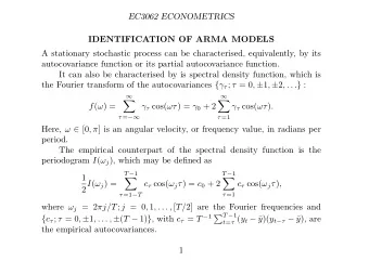
EC3062 ECONOMETRICS The Autocovariances of a Moving-Average Process Consider γ τ = E ( y t y t − τ ) � � � � = E µ i ε t − i µ j ε t − τ − j (8) i j � � = µ i µ j E ( ε t − i ε t − τ − j ) . i j Since ε ( t ) is a sequence of independently and identically distributed random variables with zero expectations, it follows that � 0 , if i � = τ + j ; (9) E ( ε t − i ε t − τ − j ) = σ 2 ε , if i = τ + j . Therefore � γ τ = σ 2 (10) µ j µ j + τ . ε j 4

EC3062 ECONOMETRICS Now let τ = 0 , 1 , . . . , q . This gives γ 0 = σ 2 ε ( µ 2 0 + µ 2 1 + · · · + µ 2 q ) , γ 1 = σ 2 ε ( µ 0 µ 1 + µ 1 µ 2 + · · · + µ q − 1 µ q ) , (11) . . . γ q = σ 2 ε µ 0 µ q . Also, γ τ = 0 for all τ > q . The first-order moving-average process y ( t ) = ε ( t ) − θε ( t − 1) has the following autocovariances: γ 0 = σ 2 ε (1 + θ 2 ) , γ 1 = − σ 2 (12) ε θ, γ τ = 0 if τ > 1 . 5

EC3062 ECONOMETRICS For a vector y = [ y 0 , y 2 , . . . , y T − 1 ] ′ of T consecutive elements from a first- order moving-average process, the dispersion matrix is 1 + θ 2 − θ 0 . . . 0 ⎡ ⎤ 1 + θ 2 − θ − θ . . . 0 ⎢ ⎥ 1 + θ 2 0 − θ . . . 0 D ( y ) = σ 2 ⎢ ⎥ (13) . ⎢ ⎥ ε . . . . ... . . . . ⎢ ⎥ . . . . ⎣ ⎦ 1 + θ 2 0 0 0 . . . In general, the dispersion matrix of a q th-order moving-average process has q subdiagonal and q supradiagonal bands of nonzero elements and zero elements elsewhere. The empirical autocovariance of lag τ ≤ T − 1 is T − τ T − 1 c τ = 1 y = 1 � � ( y t − ¯ y )( y t + τ − ¯ y ) with ¯ y t . T T t =0 t =0 Notice that c T − 1 = T − 1 y 0 y T − 1 comprises only the first and the last ele- ment of the sample. 6

EC3062 ECONOMETRICS 4 2 0 0 − 2 − 4 − 6 0 25 50 75 100 125 The graph of 125 observations on a simulated series Figure 1. generated by an MA(2) process y ( t ) = (1 + 1 . 25 L + 0 . 80 L 2 ) ε ( t ) . 7

EC3062 ECONOMETRICS 1.00 0.75 0.50 0.25 0.00 − 0.25 0 5 10 15 20 25 The theoretical autocorrelations of the MA(2) process Figure 2. y ( t ) = (1 + 1 . 25 L + 0 . 80 L 2 ) ε ( t ) (the solid bars) together with their empirical counterparts, calculated from a simulated series of 125 val- ues. 8

EC3062 ECONOMETRICS Autoregressive Processes The p th-order autoregressive AR( p ) process, is defined by (17) α 0 y ( t ) + α 1 y ( t − 1) + · · · + α p y ( t − p ) = ε ( t ) . Setting α 0 = 1 identifies y ( t ) as the output. This can be written as α ( L ) = α 0 + α 1 L + · · · + α p L p . α ( L ) y ( t ) = ε ( t ) , where For the process to be stationary, the roots of the equation α ( z ) = α 0 + α 1 z + · · · + α p z p = 0 must lie outside the unit circle. This condition enables us to write the autoregressive process as an infinite-order moving-average process in the form of y ( t ) = α − 1 ( L ) ε ( t ) . 9

EC3062 ECONOMETRICS Example. Consider the AR(1) process defined by ε ( t ) = y ( t ) − φy ( t − 1) (18) = (1 − φL ) y ( t ) . Provided that the process is stationary with | φ | < 1, it can be represented in moving-average form as 1 ε ( t ) + φε ( t − 1) + φ 2 ε ( t − 2) + · · · � � (19) y ( t ) = 1 − φLε ( t ) = . The autocovariances of the AR(1) process can be found in the manner of an MA process. Thus γ τ = E ( y t y t − τ ) � � � � φ i ε t − i φ j ε t − τ − j = E (20) i j � � φ i φ j E ( ε t − i ε t − τ − j ); = i j 10

EC3062 ECONOMETRICS Since � 0 , if i � = τ + j ; (9) E ( ε t − i ε t − τ − j ) = σ 2 ε , if i = τ + j , it follows that φ j φ j + τ = σ 2 ε φ τ � γ τ = σ 2 (21) 1 − φ 2 . ε j For a vector y = [ y 0 , y 2 , . . . , y T − 1 ] ′ of T consecutive elements from a first- order autoregressive process, the dispersion matrix has the form φ 2 φ T − 1 1 φ . . . ⎡ ⎤ φ T − 2 φ 1 φ . . . σ 2 ⎢ ⎥ φ 2 φ T − 3 φ 1 . . . ε ⎢ ⎥ (22) D ( y ) = . ⎢ ⎥ 1 − φ 2 . . . . ... ⎢ ⎥ . . . . . . . . ⎣ ⎦ φ T − 1 φ T − 2 φ T − 3 . . . 1 11

EC3062 ECONOMETRICS The Autocovariances of an Autoregressive Process Multiplying � i α i y t − i = ε t by y t − τ and taking expectations gives � (24) α i E ( y t − i y t − τ ) = E ( ε t y t − τ ) . i Taking account of the normalisation α 0 = 1, we find that � σ 2 ε , if τ = 0; (25) E ( ε t y t − τ ) = 0 , if τ > 0. Therefore, on setting E ( y t − i y t − τ ) = γ τ − i , equation (24) gives � σ 2 ε , if τ = 0; � (26) α i γ τ − i = 0 , if τ > 0. i The second equation enables us to generate the sequence { γ p , γ p +1 , . . . } given p starting values γ 0 , γ 1 , . . . , γ p − 1 . 12

EC3062 ECONOMETRICS According to (26), there is α 0 γ τ + α 1 γ τ − 1 + · · · + α 2 γ τ − p = 0 for τ > 0 Thus, given γ τ − 1 , γ τ − 2 , . . . , γ τ − p for τ ≥ p , we can find γ τ = − α 1 γ τ − 1 − α 2 γ τ − 2 − · · · − α p γ τ − p . By letting τ = 0 , 1 , . . . , p in (26), we generate a set of p +1 equations, which can be arrayed in matrix form as follows: γ 0 γ 1 γ 2 . . . γ p σ 2 1 ⎡ ⎤ ⎡ ⎤ ⎡ ⎤ ε γ 1 γ 0 γ 1 . . . γ p − 1 α 1 0 ⎢ ⎥ ⎢ ⎥ ⎢ ⎥ γ 2 γ 1 γ 0 . . . γ p − 2 α 2 0 ⎢ ⎥ ⎢ ⎥ ⎢ ⎥ (27) = . ⎢ ⎥ ⎢ ⎥ ⎢ ⎥ . . . . . . ... . ⎢ ⎥ ⎢ . ⎥ ⎢ ⎥ . . . . . . . . . . ⎣ ⎦ ⎣ ⎦ ⎣ ⎦ 0 α p γ p γ p − 1 γ p − 2 . . . γ 0 These the Yule–Walker equations, which can be used for generating the values γ 0 , γ 1 , . . . , γ p from the values α 1 , . . . , α p , σ 2 ε or vice versa. 13

EC3062 ECONOMETRICS Example. For an example of the two uses of the Yule–Walker equations, consider the AR(2) process. In this case, γ 2 ⎡ ⎤ ⎡ ⎤ ⎡ ⎤ ⎡ ⎤ γ 0 γ 1 γ 2 α 0 α 2 α 1 α 0 0 0 γ 1 ⎢ ⎥ ⎦ = γ 1 γ 0 γ 1 α 1 0 α 2 α 1 α 0 0 γ 0 ⎢ ⎥ ⎣ ⎦ ⎣ ⎣ ⎦ ⎢ ⎥ γ 2 γ 1 γ 0 α 2 0 0 α 2 α 1 α 0 γ 1 ⎣ ⎦ (28) γ 2 σ 2 ⎡ ⎤ ⎡ ⎤ ⎡ ⎤ α 0 α 1 α 2 γ 0 ε ⎦ = ⎦ . = α 1 α 0 + α 2 0 γ 1 0 ⎣ ⎦ ⎣ ⎣ α 2 α 1 α 0 γ 2 0 Given α 0 = 1 and the values for γ 0 , γ 1 , γ 2 , we can find σ 2 ε and α 1 , α 2 . Conversely, given α 0 , α 1 , α 2 and σ 2 ε , we can find γ 0 , γ 1 , γ 2 . Notice how the matrix following the first equality is folded across the axis which divides it vertically to give the matrix which follows the second equality. 14