EC3062 ECONOMETRICS IDENTIFICATION OF ARMA MODELS A stationary - PowerPoint PPT Presentation
EC3062 ECONOMETRICS IDENTIFICATION OF ARMA MODELS A stationary stochastic process can be characterised, equivalently, by its autocovariance function or its partial autocovariance function. It can also be characterised by is spectral density
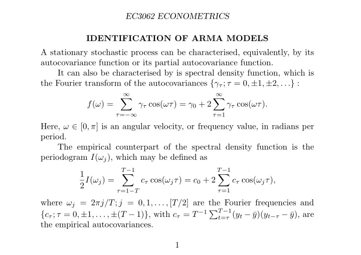
EC3062 ECONOMETRICS IDENTIFICATION OF ARMA MODELS A stationary stochastic process can be characterised, equivalently, by its autocovariance function or its partial autocovariance function. It can also be characterised by is spectral density function, which is the Fourier transform of the autocovariances { γ τ ; τ = 0 , ± 1 , ± 2 , . . . } : ∞ ∞ � � f ( ω ) = γ τ cos( ωτ ) = γ 0 + 2 γ τ cos( ωτ ) . τ = −∞ τ =1 Here, ω ∈ [0 , π ] is an angular velocity, or frequency value, in radians per period. The empirical counterpart of the spectral density function is the periodogram I ( ω j ), which may be defined as T − 1 T − 1 1 � � 2 I ( ω j ) = c τ cos( ω j τ ) = c 0 + 2 c τ cos( ω j τ ) , τ =1 τ =1 − T where ω j = 2 πj/T ; j = 0 , 1 , . . . , [ T/ 2] are the Fourier frequencies and { c τ ; τ = 0 , ± 1 , . . . , ± ( T − 1) } , with c τ = T − 1 � T − 1 t = τ ( y t − ¯ y )( y t − τ − ¯ y ), are the empirical autocovariances. 1
EC3062 ECONOMETRICS The Periodogram and the Autocovariances We need to show this definition of the peridogram is equivalent to the previous definition, which was based on the following frequency decompo- sition of the sample variance: [ T/ 2] T − 1 1 y ) 2 = 1 � � ( α 2 j + β 2 ( y t − ¯ j ) , T 2 t =0 j =0 where α j = 2 y t cos( ω j t ) = 2 � � ( y t − ¯ y ) cos( ω j t ) , T T t t β j = 2 y t sin( ω j t ) = 2 � � ( y t − ¯ y ) sin( ω j t ) . T T t t Substituting these into the term T ( α 2 j + β 2 j ) / 2 gives the periodogram �� T − 1 � T − 1 � 2 � 2 � I ( ω j ) = 2 � � cos( ω j t )( y t − ¯ y ) + sin( ω j t )( y t − ¯ y ) . T t =0 t =0 2
EC3062 ECONOMETRICS The quadratic terms may be expanded to give � � � I ( ω j ) = 2 � cos( ω j t ) cos( ω j s )( y t − ¯ y )( y s − ¯ y ) T t s + 2 � � � � sin( ω j t ) sin( ω j s )( y t − ¯ y )( y s − ¯ y ) , T t s Since cos( A ) cos( B ) + sin( A ) sin( B ) = cos( A − B ), this can be written as � � � I ( ω j ) = 2 � cos( ω j [ t − s ])( y t − ¯ y )( y s − ¯ y ) T t s On defining τ = t − s and writing c τ = � t ( y t − ¯ y )( y t − τ − ¯ y ) /T , we can reduce the latter expression to T − 1 � I ( ω j ) = 2 cos( ω j τ ) c τ , τ =1 − T which is a Fourier transform of the empirical autocovariances. 3
EC3062 ECONOMETRICS 10 7.5 5 2.5 0 0 π /4 π /2 3 π /4 π Figure 1. The spectral density function of an MA(2) process y ( t ) = (1 + 1 . 250 L + 0 . 800 L 2 ) ε ( t ) . 4
EC3062 ECONOMETRICS 60 40 20 0 0 π /4 π /2 3 π /4 π Figure 2. The graph of a periodogram calculated from 160 observations on a simulated series generated by an MA(2) process y ( t ) = (1 + 1 . 250 L + 0 . 800 L 2 ) ε ( t ). 5
EC3062 ECONOMETRICS 30 20 10 0 0 π /4 π /2 3 π /4 π Figure 3. The spectral density function of an AR(2) process (1 − 0 . 273 L + 0 . 810 L 2 ) y ( t ) = ε ( t ). 6
EC3062 ECONOMETRICS 125 100 75 50 25 0 0 π /4 π /2 3 π /4 π Figure 4. The graph of a periodogram calculated from 160 observations on a simulated series generated by an AR(2) process (1 − 0 . 273 L + 0 . 810 L 2 ) y ( t ) = ε ( t ). 7
EC3062 ECONOMETRICS 60 40 20 0 0 π /4 π /2 3 π /4 π Figure 5. The spectral density function of an ARMA(2, 1) process (1 − 0 . 273 L + 0 . 810 L 2 ) y ( t ) = (1 + 0 . 900 L ) ε ( t ). 8
EC3062 ECONOMETRICS 100 75 50 25 0 0 π /4 π /2 3 π /4 π Figure 6. The graph of a periodogram calculated from 160 observations on a simulated series generated by an ARMA(2, 1) process (1 − 0 . 273 L + 0 . 810 L 2 ) y ( t ) = (1 + 0 . 900 L ) ε ( t ). 9
EC3062 ECONOMETRICS The Methodology of Box and Jenkins Box and Jenkins proposed to use the autocorrelation and partial autocor- relation functions for identifying the orders of ARMA models. They paid little attention to the periodogram. Autocorrelation function (ACF). Given a sample y 0 , y 1 , . . . , y T − 1 of T observations, the sample autocorrelation function { r τ } is the sequence r τ = c τ /c 0 , τ = 0 , 1 , . . . , where c τ = T − 1 � ( y t − ¯ y )( y t − τ − ¯ y ) is the empirical autocovariance at lag τ and c 0 is the sample variance. As the lag increases, the number of observations comprised in the empirical autocovariances diminishes. Partial autocorrelation function (PACF). The sample partial au- tocorrelation function { p τ } gives the correlation between the two sets of residuals obtained from regressing the elements y t and y t − τ on the set of intervening values y t − 1 , y t − 2 , . . . , y t − τ +1 . The partial autocorrelation measures the dependence between y t and y t − τ after the effect of the in- tervening values has been removed. 10
EC3062 ECONOMETRICS Reduction to Stationarity. The first step is to examine the plot of the data to judge whether or not the process is stationary. A trend can be removed by fitting a parametric curve or a spline function to create a stationary sequence of residuals to which an ARMA model can be applied. Box and Jenkins believed that many empirical series can be modelled by taking a sufficient number of differences to make it stationary. Thus, the process might be modelled by the ARIMA( p, d, q ) equation α ( L ) ∇ d y ( t ) = µ ( L ) ε ( t ) , where ∇ d = ( I − L ) d is the d th power of the difference operator. Then, z ( t ) = ∇ d y ( t ) will be described by a stationary ARMA( p, q ) model. The inverse operator ∇ − 1 is the summing or integrating operator, which is why the model described an autoregressive integrated moving- average. 11
EC3062 ECONOMETRICS 18.5 18.0 17.5 17.0 16.5 16.0 15.5 0 50 100 150 Figure 7. The plot of 197 concentration readings from a chemical process taken at 2-hour intervals. 12
EC3062 ECONOMETRICS 1.00 0.75 0.50 0.25 0.00 0 5 10 �15 20 25 Figure 8. The autocorrelation function of the concentration readings from a chemical process. 13
EC3062 ECONOMETRICS 1.00 0.75 0.50 0.25 0.00 − 0.25 − 0.50 0 5 10 15 20 25 Figure 9. The autocorrelation function of the differences of the con- centration readings from the chemical process. 14
EC3062 ECONOMETRICS When Stationarity has been achieved, the autocorrelation sequence of the resulting series should converge rapidly to zero as the value of the lag increases. (See Figure 9.) The characteristics of pure autoregressive and pure moving-average process are easily spotted. Those of a mixed autoregressive moving- average model are not so easily unravelled. Moving-average processes. The theoretical autocorrelation function { ρ τ } of an M( q ) process has ρ τ = 0 for all τ > q . The partial autocorre- lation function { π τ } is liable to decay towards zero gradually. To determine whether the parent autocorrelations are zero after lag q , we may use a result of Bartlett [1946] which shows that, for a sample of size T , the standard deviation of r τ is approximately 1 � 1 / 2 1 + 2( r 2 1 + r 2 2 + · · · + r 2 � √ (4) q ) for τ > q. T A measure of the scale of the autocorrelations is provided by the limits √ of ± 1 . 96 / T , which are the approximate 95% confidence bounds for the autocorrelations of a white-noise sequence. These bounds are represented by the dashed horizontal lines on the accompanying graphs. 15
EC3062 ECONOMETRICS 4 3 2 1 0 0 − 1 − 2 − 3 − 4 − 5 0 25 50 75 100 The graph of 120 observations on a simulated series Figure 10. generated by the MA(2) process y ( t ) = (1 + 0 . 90 L + 0 . 81 L 2 ) ε ( t ) . 16
EC3062 ECONOMETRICS 1.00 0.75 0.50 0.25 0.00 − 0.25 0 5 10 15 20 25 The theoretical autocorrelation function (ACF) of the Figure 11. MA(2) process y ( t ) = (1 + 0 . 90 L + 0 . 81 L 2 ) ε ( t ) (the solid bars) together with its empirical counterpart, calculated from a simulated series of 120 observations. 17
EC3062 ECONOMETRICS 1.00 0.75 0.50 0.25 0.00 − 0.25 − 0.50 − 0.75 0 5 10 15 20 25 Figure 12. The theoretical partial autocorrelation function (PACF) of the MA(2) process y ( t ) = (1+0 . 90 L +0 . 81 L 2 ) ε ( t ) (the solid bars) together with its empirical counterpart, calculated from a simulated series of 120 observations. 18
EC3062 ECONOMETRICS Autoregressive processes. The theoretical autocorrelation function { ρ τ } of an AR( p ) process obeys a homogeneous difference equation based upon the autoregressive operator α ( L ) = 1 + α 1 L + · · · + α p L p : (5) ρ τ = − ( α 1 ρ τ − 1 + · · · + α p ρ τ − p ) for all τ ≥ p. The autocorrelation sequence will be a mixture of damped exponential and sinusoidal functions. If the sequence is of a sinusoidal nature, then the presence of complex roots in the operator α ( L ) is indicated. The partial autocorrelation function { π τ } serves most clearly to iden- tify a pure AR process. An AR( p ) process has π τ = 0 for all τ > p . The significance of the values of the empirical partial autocorrelations is judged by the fact that, for a p th order process, their standard deviations √ for all lags greater that p are approximated by 1 / T . The bounds of √ ± 1 . 96 / T are plotted on the graph of the partial autocorrelation function. 19
Recommend
More recommend
Explore More Topics
Stay informed with curated content and fresh updates.
