Does the Markov decision process fit the data Testing for the Markov - PowerPoint PPT Presentation

Does the Markov decision process fit the data —Testing for the Markov property in sequential decision making Chengchun Shi 1 and Runzhe Wan 2 and Rui Song 2 and Wenbin Lu 2 and Ling Leng 3 1 London School of Economics and Political Science 2 North Carolina State University 3 Amazon 1 / 14

Sequential decision making Objective : find an optimal policy that maximizes the cumulative reward 2 / 14

Reinforcement learning (RL) RL algorithms : trust region policy optimization (Schulman et al., 2015), deep Q-network (DQN, Mnih et al., 2015), asynchronous advantage actor-critic (Minh et al., 2016), quantile regression DQN (Dabney et al., 2018). Foundations of RL: Markov decision process (MDP, Puterman, 1994): ensures the optimal policy is stationary , and is not history-dependent. π opt depends only on S t ∪ { ( S j , A j ) } j < t only through S t ; t = π opt for any t . π opt t Markov assumption (MA): conditional on the present, the future and the past are independent, S t +1 ⊥ ⊥ { ( S j , A j ) } j < t | S t , A t . The Markov transition kernel is homogeneous in time. 3 / 14

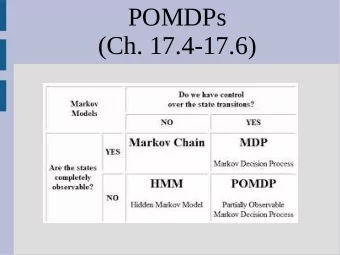
RL models Figure: Causal diagrams for MDPs, HMDPs and POMDPs. The solid lines represent the causal relationships and the dashed lines indicate the information needed to implement the optimal policy. { H t } t denotes latent variables. 4 / 14

Our contributions Methodologically propose a forward-backward learning procedure to test MA; first work on developing consistent tests for MA in RL; sequentially apply the proposed test for RL model selection : For under-fitted models, any stationary policy is not optimal; For over-fitted models, the estimated policy might be very noisy due to the inclusion of many irrelevant lagged variables. Empirically identify the optimal policy in high-order MDPs; detect partially observable MDPs. Theoretically prove our test controls type-I error under a bidirectional asymptotic framework. 5 / 14

Applications in high-order MDPs Data : the OhioT1DM dataset (Marling & Bunescu, 2018). Measurements for 6 patients with type I diabetes over 8 weeks. One-hour interval as a time unit. State : patients’ time-varying variables, e.g., glucose levels. Action : to inject insulin or not. Reward : the Index of Glycemic Control (Rodbard, 2009). 6 / 14

Applications in high-order MDPs (Cont’d) Analysis I : sequentially apply our test to determine the order of MDP; conclude it is a fourth-order MDP. Analysis II : split the data into training/testing samples; policy optimization based on fitted-Q iteration (Ernst et al., 2005), by assuming it is a k -th order MDP for k = 1 , · · · , 10; policy evaluation based on fitted-Q evaluation (Le et al., 2019); use random forest to model the Q-function; repeat the above procedure to compute the average value of policies computed under each MDP model assumption. order 1 2 3 4 5 6 7 8 9 10 value -90.8 -57.5 -63.8 -52.6 -56.2 -60.1 -63.7 -54.9 -65.1 -59.6 7 / 14

Applications in partially observable MDPs 8 / 14

Applications in partially observable MDPs (Cont’d) Empirical rejection rates under the alternative hypothesis (MA is violated). α = (0 . 05 , 0 . 1) from left to right. Empirical rejection rates under the null hypothesis (MA holds). α = (0 . 05 , 0 . 1) from left to right. 9 / 14

Forward-backward learning Challenge: develop a valid test for MA in moderate or high-dimensions (no existing method works well); the dimension of the state increases as we concatenate measurements over multiple time points in order to test for a high-order MDP. This motivates our forward-backward learning procedure. 10 / 14

Forward-backward learning (Cont’d) Some key components of our algorithm: Characterize MA based on the notion of conditional characteristic function (CCF); To deal with moderate or high-dimensional state space, employ modern machine learning (ML) algorithms to estimate CCF: Learn CCF of S t +1 given A t and S t ( forward learner ); Learn CCF of ( S t , A t ) given ( S t +1 , A t +1 ) ( backward learner ); Develop a random forest-based algorithm to estimate CCF; Borrow ideas from the quantile random forest algorithm (Meinshausen, 2006) to facilitate the computation. To alleviate the bias of ML algorithms, construct doubly-robust estimating equations by integrating forward and backward learners; To improve the power, construct a maximum-type test statistic; To control the type-I error, approximate the distribution of our test via multiplier bootstrap . 11 / 14

Bidirectional theory N the number of trajectories; T the number of decision points in each trajectory; bidirectional asymptotics: a framework where either N or T grows to ∞ ; large T , small N (mobile health) large N , small T (some medical studies) large N , large T (games) 12 / 14

Bidirectional theory (cont’d) (C1) Actions are generated by a fixed behavior policy. (C2) The process { S t } t ≥ 0 is exponentially β -mixing. (C3) The ℓ 2 prediction errors of forward and backward learners converge at a rate faster than ( NT ) − 1 / 4 . Theorem Assume (C1)-(C3) hold. Then under some other mild conditions, our test controls the type-I error asymptotically as either N or T diverges to ∞ . 13 / 14

Thanks! The paper is accepted at ICML 2020. Preprint https://arxiv.org/pdf/2006.02615.pdf , Python code TestMDP https://github.com/RunzheStat/TestMDP 14 / 14