Discriminative vs. Generative Learning CS 760@UW-Madison Goals for - PowerPoint PPT Presentation

Discriminative vs. Generative Learning CS 760@UW-Madison

Goals for the lecture you should understand the following concepts • the relationship between logistic regression and Naïve Bayes • the relationship between discriminative and generative learning • when discriminative/generative is likely to learn more accurate models

Review

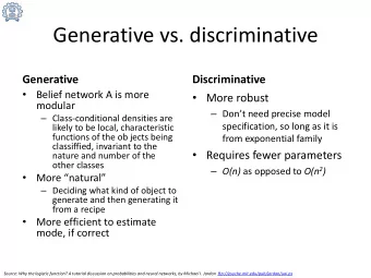
Discriminative vs. Generative Discriminative approach: • hypothesis ℎ ∈ 𝐼 directly predicts the label given the features 𝑧 = ℎ(𝑦) or more generally, 𝑞 𝑧 𝑦 = ℎ(𝑦) • then define a loss function 𝑀(ℎ) and find hypothesis with min. loss Generative approach: • hypothesis ℎ ∈ 𝐼 specifies a generative story for how the data was created: 𝑞(𝑦, 𝑧) = ℎ(𝑦, 𝑧) • then pick a hypothesis by maximum likelihood estimation (MLE) or Maximum A Posteriori (MAP)

Summary: generative approach • Step 1: specify the joint data distribution (generative story) • Step 2: use MLE or MAP for training • Step 3: use Bayes’ rule for inference on test instances • Example: Naïve Bayes (conditional independence) 𝑞 𝑦, 𝑧 = 𝑞 𝑧 𝑞 𝑦 𝑧 = 𝑞 𝑧 ෑ 𝑞(𝑦 𝑗 |𝑧) 𝑗

Summary: discriminative approach • Step 1: specify the hypothesis class • Step 2: specify the loss • Step 3: design optimization algorithm for training How to design the hypotheses and the loss? Can design by a generative approach! • Step 0: specify 𝑞 𝑦 𝑧 and 𝑞(𝑧) • Step 1: compute hypotheses 𝑞(𝑧|𝑦) using Bayes’ rule • Step 2: use conditional MLE to derive the negative log- likelihood loss (or use MAP to derive the loss) • Step 3: design optimization algorithm for training • Example: logistic regression

Logistic regression • Suppose the class-conditional densities 𝑞 𝑦 𝑧 is normal 2𝜌 𝑒/2 exp − 1 1 2 𝑞 𝑦 𝑧 = 𝑞 𝑦 𝑍 = 𝑧 = 𝑂 𝑦|𝜈 𝑧 , 𝐽 = 𝑦 − 𝜈 𝑧 2 • Then conditional probability by Bayes’ rule: exp(𝑏 𝑧 ) 𝑞 𝑦|𝑍 = 𝑧 𝑞(𝑍 = 𝑧) 𝑞 𝑍 = 𝑧|𝑦 = σ 𝑙 𝑞 𝑦|𝑍 = 𝑙 𝑞(𝑍 = 𝑙) = σ 𝑙 exp(𝑏 𝑙 ) where 𝑈 = − 1 2 𝑦 𝑈 𝑦 + 𝑥 𝑙 𝑦 + 𝑐 𝑙 𝑏 𝑙 ≔ ln 𝑞 𝑦 𝑍 = 𝑙 𝑞 𝑍 = 𝑙 with 𝑐 𝑙 = − 1 1 𝑥 𝑙 = 𝜈 𝑙 , 𝑈 𝜈 𝑙 + ln 𝑞 𝑍 = 𝑙 + ln 2 𝜈 𝑙 2𝜌 𝑒/2

Logistic regression • Suppose the class-conditional densities 𝑞 𝑦 𝑧 is normal 2𝜌 𝑒/2 exp − 1 1 2 𝑞 𝑦 𝑧 = 𝑞 𝑦 𝑍 = 𝑧 = 𝑂 𝑦|𝜈 𝑧 , 𝐽 = 𝑦 − 𝜈 𝑧 2 1 2 𝑦 𝑈 𝑦 , we have • Cancel out − exp(𝑏 𝑧 ) 𝑥 𝑙 𝑈 𝑦 + 𝑐 𝑙 𝑞 𝑍 = 𝑧|𝑦 = σ 𝑙 exp(𝑏 𝑙 ) , 𝑏 𝑙 ≔ where 𝑐 𝑙 = − 1 1 𝑥 𝑙 = 𝜈 𝑙 , 𝑈 𝜈 𝑙 + ln 𝑞 𝑍 = 𝑙 + ln 2 𝜈 𝑙 2𝜌 𝑒/2

Logistic regression: summary • Suppose the class-conditional densities 𝑞 𝑦 𝑧 is normal 2𝜌 𝑒/2 exp − 1 1 2 𝑞 𝑦 𝑧 = 𝑞 𝑦 𝑍 = 𝑧 = 𝑂 𝑦|𝜈 𝑧 , 𝐽 = 𝑦 − 𝜈 𝑧 2 • Then exp( 𝑥 𝑧 𝑈 𝑦 + 𝑐 𝑧 ) 𝑞 𝑍 = 𝑧|𝑦 = σ 𝑙 exp( 𝑥 𝑙 𝑈 𝑦 + 𝑐 𝑙 ) which is the hypothesis class for multiclass logistic regression • Training: find parameters {𝑥 𝑙 , 𝑐 𝑙 } that minimize the negative log-likelihood loss 𝑛 − 1 log 𝑞 𝑧 = 𝑧 (𝑘) 𝑦 (𝑘) 𝑛 ෍ 𝑘=1

Naïve Bayes vs. Logistic Regression

Connecting Naïve Bayes and logistic regression • Interesting observation: logistic regression is derived from the generative story 2𝜌 𝑒/2 exp − 1 1 2 𝑞 𝑦 𝑧 = 𝑞 𝑦 𝑍 = 𝑧 = 𝑂 𝑦|𝜈 𝑧 , 𝐽 = 𝑦 − 𝜈 𝑧 2 1 exp − 1 2 = 2𝜌 𝑒/2 ෑ 2 𝑦 𝑗 − 𝑣 𝑧𝑗 𝑗 which is a special case of Naïve Bayes! • Is the general Naïve Bayes assumption enough to get logistic regression? (Instead of the more special Normal distribution assumption) • Yes, with an additional linearity assumption

Naïve Bayes revisited consider Naïve Bayes for a binary classification task n  = = ( 1 ) ( | 1 ) P Y P x Y i = = = 1 ( 1 | ,..., ) i P Y x x 1 n ( ,..., ) P x x 1 n n  expanding denominator = = ( 1 ) ( | 1 ) P Y P x Y i = = 1 i n n   = = + = = ( 1 ) ( | 1 ) ( 0 ) ( | 0 ) P Y P x Y P Y P x Y i i = = 1 1 i i dividing everything by numerator 1 = n  = = ( 0 ) ( | 0 ) P Y P x Y i + = 1 1 i n  = = ( 1 ) ( | 1 ) P Y P x Y i = 1 i

Naïve Bayes revisited 1 = = ( 1 | ,..., ) P Y x x 1 n n  = = ( 0 ) ( | 0 ) P Y P x Y i + = 1 1 i n  = = ( 1 ) ( | 1 ) P Y P x Y i = 1 i 1 = applying exp(ln( a )) = a     n    = =   ( 0 ) ( | 0 ) P Y P x Y i     + = 1 1 exp ln i     n  = =  ( 1 ) ( | 1 )   P Y P x Y  i     = 1 i 1 applying ln(a/b) = -ln(b/a) =     n     = =  ( 1 ) ( | 1 ) P Y P x Y i     + − = 1 1 exp ln i     n  = =  ( 0 ) ( | 0 )   P Y P x Y  i     = 1 i

Naïve Bayes revisited 1 = = ( 1 | ,..., ) P Y x x 1   n   n    = =   ( 1 ) ( | 1 ) P Y P x Y i     + − = 1 1 exp ln i     n  = =  ( 0 ) ( | 0 )   P Y P x Y  i     = 1 i converting log of products to sum of logs 1 = = ( 1 | ,..., ) P Y x x 1   n    =  = n ( 1 ) ( | 1 ) P Y  P x Y   + − −     1 exp ln ln i     = =   ( 0 )  ( | 0 )   P Y P x Y  = 1 i i Does this look familiar?

Naïve Bayes vs. logistic regression Naïve Bayes 1 = = ( 1 | ,..., ) P Y x x   1 n    =  = n ( 1 ) ( | 1 ) P Y  P x Y     + −   − i 1 exp ln ln     = =  ( 0 )  ( | 0 )    P Y P x Y  = 1 i i Linearity assumption: logistic regression the log-ratio is linear in 𝑦 1 = ( ) f x     n    + − +   1 exp w w i x   0 i     = 1 i

Naïve Bayes vs. logistic regression Naïve Bayes 1 = = ( 1 | ,..., ) P Y x x   1 n    =  = n ( 1 ) ( | 1 ) P Y  P x Y     + −   − i 1 exp ln ln     = =  ( 0 )  ( | 0 )    P Y P x Y  = 1 i i Linearity assumption: logistic regression the log-ratio is linear in 𝑦 1 = ( ) f x     n    + − +   1 exp w w i x   0 i     = 1 i Summary: If we begin with a Naïve Bayes generative story to derive a discriminative approach (assuming linearity), we get logistic regression!

Naïve Bayes vs. logistic regression Naïve Bayes Generative counterpart of logistic regression 1 = = ( 1 | ,..., ) P Y x x   1 n    =  = n ( 1 ) ( | 1 ) P Y  P x Y     + −   − i 1 exp ln ln     = =  ( 0 )  ( | 0 )    P Y P x Y  = 1 i i Discriminative counterpart of Naïve Bayes logistic regression 1 = ( ) f x     n    + − +   1 exp w w i x   0 i     = 1 i Summary: If we begin with a Naïve Bayes generative story to derive a discriminative approach (assuming linearity), we get logistic regression!

Naïve Bayes vs. logistic regression Conditional Independence (Naïve Bayes assumption) Generative approach Discriminative approach (+ linearity assumption) Naïve Bayes method Logistic regression

Logistic regression as a neural net ln P ( Y = 1) æ ö ÷ ç è P ( Y = 0) ø Y 1 ln P ( red | Y = 1) æ ö ÷ ç è P ( red | Y = 0) ø Color=red Color=blue Size=big Size=small ln P ( blue | Y = 1) æ ö ÷ ç è P ( blue | Y = 0) ø The connection can give interpretation for the weights in logistic regression: weights correspond to log ratios

Which is better?

Naïve Bayes vs. logistic regression • they have the same functional form, and thus have the same hypothesis space bias (recall our discussion of inductive bias) • Do they learn the same models? In general, no . They use different methods to estimate the model parameters. Naïve Bayes uses MLE to learn the parameters 𝑞(𝑦 𝑗 |𝑧) , whereas LR minimizes the loss to learn the parameters 𝑥 𝑗 .