Generative and discriminative classification techniques Machine - PowerPoint PPT Presentation
Generative and discriminative classification techniques Machine Learning and Category Representation 2013-2014 Jakob Verbeek, December 13+20, 2013 Course website: http://lear.inrialpes.fr/~verbeek/MLCR.13.14 Classification apple pear tomato
Generative and discriminative classification techniques Machine Learning and Category Representation 2013-2014 Jakob Verbeek, December 13+20, 2013 Course website: http://lear.inrialpes.fr/~verbeek/MLCR.13.14
Classification apple pear tomato cow ? dog hor se Given: training images and their categories To which category does a new image belong?
Classification Goal is to predict for a test data input the corresponding class label. – Data input x , eg. image but could be anything , format may be vector or other – Class label y , can take one out of at least 2 discrete values, can be more In binary classification we often refer to one class as “positive”, and the ► other as “negative” Classifier: function f(x) that assigns a class to x, or probabilities over the classes. Training data: pairs (x,y) of inputs x, and corresponding class label y. Learning a classifier: determine function f(x) from some family of functions based on the available training data. Classifier partitions the input space into regions where data is assigned to a given class – Specific form of these boundaries will depend on the family of classifiers used
Discriminative vs generative methods Generative probabilistic methods – Model the density of inputs x from each class p(x|y) – Estimate class prior probability p(y) – Use Bayes’ rule to infer distribution over class given input p ( y ∣ x )= p ( y ) p ( x ∣ y ) p ( x )= ∑ y p ( y ) p ( x ∣ y ) p ( x ) Discriminative (probabilistic) methods Directly estimate class probability given input: p(y|x) ► Some methods do not have probabilistic interpretation, ► eg. they fit a function f(x), and assign to class 1 if f(x)>0, and to class 2 if f(x)<0
Generative classification methods Generative probabilistic methods – Model the density of inputs x from each class p(x|y) – Estimate class prior probability p(y) – Use Bayes’ rule to infer distribution over class given input p ( y ∣ x )= p ( y ) p ( x ∣ y ) p ( x )= ∑ y p ( y ) p ( x ∣ y ) p ( x ) 1. Selection of model class: – Parametric model: Gaussian (for continuous), Bernoulli (for binary), … – Semi-parametric models: mixtures of Gaussian / Bernoulli / … – Non-parametric models: histograms, nearest-neighbor method, … 2. Estimate parameters of density for each class to obtain p(x|y) – Eg: run EM to learn Gaussian mixture on data of each class 3. Estimate prior probability of each class – If data point is equally likely given each class, then assign to the most probable class. – Prior probability might be different than the number of available examples !
Generative classification methods Generative probabilistic methods – Model the density of inputs x from each class p(x|y) – Estimate class prior probability p(y) – Use Bayes’ rule to predict classes given input p ( y ∣ x )= p ( y ) p ( x ∣ y ) p ( x )= ∑ y p ( y ) p ( x ∣ y ) p ( x ) Given class conditional model, classification is trivial: just apply Bayes’ rule – Compute p(x|class) for each class, – multiply with class prior probability – Normalize to obtain the class probabilities Adding new classes can be done by adding a new class conditional model Existing class conditional models stay as they are ► Estimate p(x|new class) from training examples of new class ► Re-estimate class prior probabilities ►
Generative classification methods Generative probabilistic methods – Model the density of inputs x from each class p(x|y) – Estimate class prior probability p(y) – Use Bayes’ rule to predict classes given input p ( y ∣ x )= p ( y ) p ( x ∣ y ) p ( x )= ∑ y p ( y ) p ( x ∣ y ) p ( x ) • Three-class example in 2d with parametric model – Single Gaussian model per class, equal mixing weights – Exercise: characterize surface of equal class probability when the covariance matrices are all equal p(x|y) p(y|x)
Generative classification methods Generative probabilistic methods – Model the density of inputs x from each class p(x|y) – Estimate class prior probability p(y) – Use Bayes’ rule to infer distribution over class given input 1. Selection of model class: – Parametric model: Gaussian (for continuous), Bernoulli (for binary), … – Semi-parametric models: mixtures of Gaussian, mixtures of Bernoulli, … – Non-parametric models: histograms, nearest-neighbor method, … 1. Estimate parameters of density for each class to obtain p(x|class) – Eg: run EM to learn Gaussian mixture on data of each class 1. Estimate prior probability of each class – Fraction of points in training data for each class – Assumes class proportions in train data are representative for test time (not always true)
Histogram density estimation Suppose we – have N data points – use a histogram with C cells How to set the density level in each cell ? – Maximum likelihood estimator. – Proportional to nr of points n in cell – Inversely proportional to volume V of cell p c = n c NV c Exercise: derive this result ► Problems with histogram method: – # cells scales exponentially with the dimension of the data – Discontinuous density estimate – How to choose cell size?
The ‘curse of dimensionality’ Number of bins increases exponentially with the dimensionality of the data. – Fine division of each dimension: many empty bins – Rough division of each dimension: poor density model The number of parameters may be reduced by assuming independence between the dimensions of x : the naïve Bayes model D p ( x )= ∏ d = 1 d ) p ( x – For example, for histogram model: we estimate a histogram per dimension – Still C D cells, but only D x C parameters to estimate, instead of C D Model is “naïve” since it assumes that all variables are independent… Unrealistic for high dimensional data, where variables tend to be dependent ► Typically poor density estimator for p(x|y) ► Classification performance may still be good using the derived p(y|x) ► Principle can be applied to estimation with any type of model
k -nearest-neighbor density estimation Instead of having fixed cells as in histogram method, put a cell around the test sample we want to know p(x) for – fix number of samples in the cell, find the right cell size. Probability to find a point in a sphere A centered on x 0 with volume v is P ( x ∈ A )= ∫ A p ( x ) dx A smooth density is approximately constant in small region, and thus P ( x ∈ A )= ∫ A p ( x ) dx ≈ v p ( x 0 ) Alternatively: estimate P from the fraction of training data in A P ( x ∈ A )≈ k – Total N data points, k in the sphere A N p ( x 0 )≈ k Combine the above to obtain estimate Nv – Density estimates not guaranteed to integrate to one!
k -nearest-neighbor density estimation Procedure in practice: – Choose k – For given x , compute the volume v which contain k samples. p ( x )≈ k – Estimate density with Nv 2r d π d / 2 Volume of a sphere with radius r in d dimensions is v ( r ,d )= Γ( d / 2 + 1 ) What effect does k have? – Data sampled from mixture of Gaussians plotted in green – Larger k , larger region, smoother estimate Selection of k typically by cross validation
k -nearest-neighbor classification Use k -nearest neighbor density estimation to find p(x|y) Apply Bayes rule for classification: k -nearest neighbor classification p ( x )= k – Find sphere volume v to capture k data points for estimate N v p ( x ∣ y = c )= k c – Use the same sphere for each class for estimates N c v p ( y = c )= N c – Estimate class prior probabilities N – Calculate class posterior distribution as fraction of k neighbors in class c p ( y = c ∣ x )= p ( y = c ) p ( x ∣ y = c ) p ( x ) k c 1 = Nv p ( x ) = k c k
Summary generative classification methods (Semi-) Parametric models, eg p(x|y) is Gaussian, or mixture of … – Pros: no need to store training data, just the class conditional models – Cons: may fit the data poorly, and might therefore lead to poor classification result Non-parametric models: – Advantage is their flexibility: no assumption on shape of data distribution – Histograms: • Only practical in low dimensional space (<5 or so), application in high dimensional space will lead to exponentially many cells, most of which will be empty • Naïve Bayes modeling in higher dimensional cases – K-nearest neighbor density estimation: simple but expensive at test time • storing all training data (memory space) • Computing nearest neighbors (computation)
Discriminative vs generative methods Generative probabilistic methods – Model the density of inputs x from each class p(x|y) – Estimate class prior probability p(y) – Use Bayes’ rule to infer distribution over class given input Discriminative methods directly estimate class probability given input: p(y|x) Choose class of decision functions in feature space ► Estimate function to maximize performance on the training set ► Classify a new pattern on the basis of this decision rule. ►
Recommend
More recommend
Explore More Topics
Stay informed with curated content and fresh updates.
