Logistic Regression, Generative and Discriminative Classifiers - PowerPoint PPT Presentation

Logistic Regression, Generative and Discriminative Classifiers Recommended reading: • Ng and Jordan paper “On Discriminative vs. Generative classifiers: A comparison of logistic regression and naïve Bayes,” A. Ng and M. Jordan, NIPS 2002. Machine Learning 10-701 Tom M. Mitchell Carnegie Mellon University Thanks to Ziv Bar-Joseph, Andrew Moore for some slides

Overview Last lecture: • Naïve Bayes classifier • Number of parameters to estimate • Conditional independence This lecture: • Logistic regression • Generative and discriminative classifiers • (if time) Bias and variance in learning

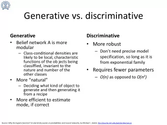
Generative vs. Discriminative Classifiers Training classifiers involves estimating f: X � Y, or P(Y|X) Generative classifiers: • Assume some functional form for P(X|Y), P(X) • Estimate parameters of P(X|Y), P(X) directly from training data • Use Bayes rule to calculate P(Y|X= x i ) Discriminative classifiers: 1. Assume some functional form for P(Y|X) 2. Estimate parameters of P(Y|X) directly from training data

• Consider learning f: X � Y, where • X is a vector of real-valued features, < X 1 … X n > • Y is boolean • So we use a Gaussian Naïve Bayes classifier • assume all X i are conditionally independent given Y • model P(X i | Y = y k ) as Gaussian N( µ ik , σ ) • model P(Y) as binomial (p) • What does that imply about the form of P(Y|X)?

• Consider learning f: X � Y, where • X is a vector of real-valued features, < X 1 … X n > • Y is boolean • assume all X i are conditionally independent given Y • model P(X i | Y = y k ) as Gaussian N( µ ik , σ ) • model P(Y) as binomial (p) • What does that imply about the form of P(Y|X)?

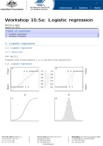
Logistic regression • Logistic regression represents the probability of category i using a linear function of the input variables: = = = + + + K ( | ) ( ) P Y i X x g w w x w x 0 1 1 i i id d where for i<k z e i = ( ) g z − i 1 K ∑ + z 1 e j = 1 j and for k 1 = ( ) g z − k 1 K ∑ + z 1 e j = 1 j

Logistic regression • The name comes from the logit transformation: = = ( | ) ( ) p Y i X x g z = = + + + i K log log w w x w x = = 0 i 1 1 id d ( | ) ( ) p Y K X x g z k

Binary logistic regression • We only need one set of parameters + + + K w w x w x e 0 1 1 d d = = = ( 1 | ) p Y X x + + + + K w w x w x 1 e 0 1 1 d d 1 = − + + + + K ( ) w w x w x 1 e 0 1 1 d d 1 = − + z 1 e • This results in a “squashing function” which turns linear predictions into probabilities

Logistic regression vs. Linear regression 1 = = = ( 1 | ) P Y X x − + z 1 e

Example

Log likelihood ∑ N = + − − ( ) log ( ; ) ( 1 ) log( 1 ( ; )) l w y p x w y p x w = i i i i 1 i ( ; ) 1 p x w ∑ N = + i log log( ) y − + = i x w 1 i ( 1 ( ; ) 1 p x w e i i ∑ N = − + x w log( 1 ) y x w e i = i i 1 i

Log likelihood ∑ N = + − − ( ) log ( ; ) ( 1 ) log( 1 ( ; )) l w y p x w y p x w = i i i i 1 i ( ; ) 1 p x w ∑ N = + i log log( ) y − + = i x w 1 i ( 1 ( ; ) 1 p x w e i i ∑ N = − + x w log( 1 ) y x w e i = i i 1 i • Note: this likelihood is a concave in w

Maximum likelihood estimation ∂ ∂ ∑ N = − + x w ( ) { log( 1 )} l w y x w e i ∂ ∂ = i i 1 i w w j j = K Common (but not only) ∑ = N − approaches: ( ( , )) x y p x w No close form = ij i i 1 i Numerical Solutions: solution! • Line Search • Simulated Annealing prediction error • Gradient Descent • Newton’s Method • Matlab glmfit function

Gradient descent

Gradient ascent ∑ + ← + ε − 1 t t ( ( ( , )) w w x y p x w j j ij i i i • Iteratively updating the weights in this fashion increases likelihood each round. • We eventually reach the maximum • We are near the maximum when changes in the weights are small. • Thus, we can stop when the sum of the absolute values of the weight differences is less than some small number.

Example • We get a monotonically increasing log likelihood of the training labels as a function of the iterations

Convergence • The gradient ascent learning method converges when there is no incentive to move the parameters in any particular direction: ∑ − = ∀ ( ( ( , )) 0 x y p x w k ij i i i • This condition means that the prediction error is uncorrelated with the components of the input vector

Naïve Bayes vs. Logistic Regression [Ng & Jordan, 2002] • Generative and Discriminative classifiers • Asymptotic comparison (# training examples � infinity) • when model correct • when model incorrect • Non-asymptotic analysis • convergence rate of parameter estimates • convergence rate of expected error • Experimental results

Generative-Discriminative Pairs Example: assume Y boolean, X = <X 1 , X 2 , …, X n >, where x i are boolean, perhaps dependent on Y, conditionally independent given Y Generative model: naïve Bayes: s indicates size of set. l is smoothing parameter Classify new example x based on ratio Equivalently, based on sign of log of this ratio

Generative-Discriminative Pairs Example: assume Y boolean, X = <x 1 , x 2 , …, x n >, where x i are boolean, perhaps dependent on Y, conditionally independent given Y Generative model: naïve Bayes: Classify new example x based on ratio Discriminative model: logistic regression Note both learn linear decision surface over X in this case

What is the difference asymptotically? Notation: let denote error of hypothesis learned via algorithm A, from m examples • If assumed model correct (e.g., naïve Bayes model), and finite number of parameters, then • If assumed model incorrect Note assumed discriminative model can be correct even when generative model incorrect, but not vice versa

Rate of covergence: logistic regression Let h Dis,m be logistic regression trained on m examples in n dimensions. Then with high probability: Implication: if we want for some constant , it suffices to pick � Convergences to its classifier, in order of n examples (result follows from Vapnik’s structural risk bound, plus fact that VCDim of n dimensional linear separators is n )

Rate of covergence: naïve Bayes Consider first how quickly parameter estimates converge toward their asymptotic values. Then we’ll ask how this influences rate of convergence toward asymptotic classification error.

Rate of covergence: naïve Bayes parameters

from UCI data experiments Some sets

What you should know: • Logistic regression – What it is – How to solve it – Log linear models • Generative and Discriminative classifiers – Relation between Naïve Bayes and logistic regression – Which do we prefer, when? • Bias and variance in learning algorithms

Acknowledgment Some of these slides are based in part on slides from previous machine learning classes taught by Ziv Bar-Joseph, Andrew Moore at CMU, and by Tommi Jaakkola at MIT. I thank them for providing use of their slides.