Optimal scaling and convergence of Markov chain Monte Carlo methods - PowerPoint PPT Presentation

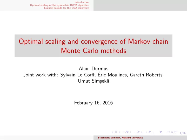
Introduction Optimal scaling of the symmetric RWM algorithm Explicit bounds for the ULA algorithm Optimal scaling and convergence of Markov chain Monte Carlo methods Alain Durmus Joint work with: Sylvain Le Corff, ´ Eric Moulines, Gareth Roberts, Umut S ¸im¸ sekli February 16, 2016 1/66 Stochastic seminar, Helsinki university

Introduction Optimal scaling of the symmetric RWM algorithm Explicit bounds for the ULA algorithm 1 Introduction 2 Optimal scaling of the symmetric RWM algorithm 3 Explicit bounds for the ULA algorithm 2/66 Stochastic seminar, Helsinki university

Introduction Optimal scaling of the symmetric RWM algorithm Explicit bounds for the ULA algorithm Introduction Sampling distributions over high-dimensional state-space has recently attracted a lot of research efforts in computational statistics and machine learning community... Applications (non-exhaustive) Bayesian inference for high-dimensional models and Bayesian non parametric. Bayesian linear inverse problems (typically function space problems). Aggregation of estimators and experts. 3/66 Stochastic seminar, Helsinki university

Introduction Optimal scaling of the symmetric RWM algorithm Explicit bounds for the ULA algorithm Bayesian setting A Bayesian model is specified by 1 a prior distribution p on the parameter space θ ∈ R d 2 the sampling distribution of the observed data conditional on its parameters, often termed likelihood: Y ∼ L ( ·| θ ) The inference is based on the posterior distribution: p (d θ ) L ( Y | θ ) π (d θ ) = L ( Y | u ) p (d u ) . � In most cases the normalizing constant is not tractable: π (d θ ) ∝ p (d θ ) L ( Y | θ ) . 4/66 Stochastic seminar, Helsinki university

Introduction Optimal scaling of the symmetric RWM algorithm Explicit bounds for the ULA algorithm Logistic and probit regression Likelihood: Binary regression set-up in which the binary observations (responses) ( Y 1 , . . . , Y n ) are conditionally independent Bernoulli random variables with success probability F ( θ T X i ) , where 1 X i is a d dimensional vector of known covariates, 2 θ is a d dimensional vector of unknown regression coefficient 3 F is a distribution function. Two important special cases: 1 probit regression: F is the standard normal distribution function, 2 logistic regression: F is the standard logistic distribution function, F ( t ) = e t / (1 + e t ) . 5/66 Stochastic seminar, Helsinki university

Introduction Optimal scaling of the symmetric RWM algorithm Explicit bounds for the ULA algorithm Logistic and probit regression (II) The posterior density distribution of θ is given, up to a proportionality constant by π ( θ | ( Y, X )) ∝ exp( − U ( θ )) , where the potential U ( θ ) is given by p { Y i log F ( θ T X i )+(1 − Y i ) log(1 − F ( θ T X i )) } +g( θ ) , � U ( θ ) = − i =1 where g is the log density of the posterior distribution. Two important cases: Gaussian prior g( θ ) = (1 / 2) θ T Σ θ , ridge regression. Laplace prior g( θ ) = λ � d i =1 | θ i | , lasso regression. 6/66 Stochastic seminar, Helsinki university

Introduction Optimal scaling of the symmetric RWM algorithm Explicit bounds for the ULA algorithm Bayesian setting (II) Bayesian decision theory relies on computing expectations: � π ( f ) = R d f ( θ ) π (d θ ) Generic problem: estimation of an integral π ( f ) , where - π is known up to a multiplicative factor ; - Sampling directly from π is not an option; n � A solution is to approximate E π [ f ] by n − 1 f ( X i ) , i =1 where ( X i ) i ≥ 0 is a Markov chain associated with a Markov kernel P for which π is invariant. 7/66 Stochastic seminar, Helsinki university

Introduction Optimal scaling of the symmetric RWM algorithm Explicit bounds for the ULA algorithm Markov chain theory Invariant probability measure: π is said to be an invariant probability measure for the Markov kernel P if X 0 ∼ π then X 1 ∼ π Ergodic Theorem (Meyn and Tweedie, 2003): If π is invariant, With some conditions on P , we have for any f ∈ L 1 ( π ) , n 1 � � f ( X i ) − → f ( x ) π ( x )d x . n π -a.s. i =1 8/66 Stochastic seminar, Helsinki university

Introduction Optimal scaling of the symmetric RWM algorithm Explicit bounds for the ULA algorithm MCMC: rationale To approximate π ( f ) : find P with invariant measure π , from which we can efficiently sample. MCMC methods are algorithms which aims to build such kernel. One of the most famous example: The Metropolis-Hastings algorithm. 9/66 Stochastic seminar, Helsinki university

Introduction Optimal scaling of the symmetric RWM algorithm Explicit bounds for the ULA algorithm The Metropolis-Hastings algorithm Initial Data: the target density π , a transition density q , X 0 ∼ µ 0 . For k ≥ 0 given X k , 1 Generate Y k +1 ∼ q ( X k , · ) . 2 Set � Y k +1 with probability α ( X k , Y k +1 ) , X k +1 = with probability 1 − α ( X k , Y k +1 ) . X k where α ( x, y ) = 1 ∧ π ( y ) q ( y, x ) q ( x, y ) . π ( x ) π is invariant for the corresponding Markov kernel P . 10/66 Stochastic seminar, Helsinki university

Introduction Optimal scaling of the symmetric RWM algorithm Explicit bounds for the ULA algorithm Example: The symmetric Random Walk Metropolis algorithm The Random Walk Metropolis:  Y k +1 = X k + σZ k +1 ( Z k ) k ≥ 0 i.i.d. sequence of law N d (0 , Id d )   = σ − d φ d ( � y − x � /σ ) where φ d is the Gaussian density on R d q ( x, y )  α ( x, y ) = π ( y ) /π ( x ) .  11/66 Stochastic seminar, Helsinki university

Introduction Optimal scaling of the symmetric RWM algorithm Explicit bounds for the ULA algorithm Study of MCMC methods: measures of efficiency 1 How to measure the efficiency of MCMC methods ? 2 Equivalent problem: quantifying the convergence of the Markov kernel P to its stationary distribution π . 3 We consider two criteria: the asymptotic variance ⇒ justifies optimal scaling results. convergence in some metric on the set of probability measures. 12/66 Stochastic seminar, Helsinki university

Introduction Optimal scaling of the symmetric RWM algorithm Explicit bounds for the ULA algorithm 1 Introduction 2 Optimal scaling of the symmetric RWM algorithm 3 Explicit bounds for the ULA algorithm 13/66 Stochastic seminar, Helsinki university

Introduction Optimal scaling of the symmetric RWM algorithm Explicit bounds for the ULA algorithm Behaviour of the RWM Recall the RWM proposal: Y k +1 = X k + σZ k +1 On the one hand, σ should be as large as possible so that the chain explores the state spaces. On the other hand, σ should not be too large as possible otherwise α → 0 . 14/66 Stochastic seminar, Helsinki university

Introduction Optimal scaling of the symmetric RWM algorithm Explicit bounds for the ULA algorithm Scaling problems Questions: How should σ depend on the dimension d ? We study the following very simple model. Consider π a one dimensional positive density on R of the form π ∝ e − u . Define the positive density on given for all x ∈ R d by d d e u ( x i ) , π d ( x ) = � � π ( x i ) = i =1 i =1 where x i is the i -th component of x . 15/66 Stochastic seminar, Helsinki university

Introduction Optimal scaling of the symmetric RWM algorithm Explicit bounds for the ULA algorithm Study of the acceptance ratio (I) Recall π d ( x ) = � d i =1 π ( x i ) = � d i =1 e u ( x i ) Then the acceptance ratio can be written of the form for all x, y ∈ R d , α ( x, y ) = 1 ∧ π ( y ) π ( x ) � d � � = 1 ∧ exp u ( x i ) − u ( y i ) . i =1 16/66 Stochastic seminar, Helsinki university

Introduction Optimal scaling of the symmetric RWM algorithm Explicit bounds for the ULA algorithm Study of the acceptance ratio (II) �� d � Recall α ( x, y ) = 1 ∧ exp i =1 u ( x i ) − u ( y i ) We want that the acceptance ratio during the algorithm ∈ (0 , 1) . 0 ∼ π d and the proposal based on X d Let X d 0 , Y d 1 = X d 0 + σZ d 1 . We consider the mean acceptance ratio, i.e. the quantity: α ( X d 0 , Y d α ( X d 0 , X d 0 + σZ d � � � � E 1 ) = E 1 ) � d � �� � u ( X d 0 ,i ) − u ( X d 0 ,i + σZ d 1 ∧ exp = E 1 ,i ) . i =1 17/66 Stochastic seminar, Helsinki university

Introduction Optimal scaling of the symmetric RWM algorithm Explicit bounds for the ULA algorithm Study of the acceptance ratio (III) � �� d �� � α ( X d 0 , Y d � i =1 u ( X d 0 ,i ) − u ( X d 0 ,i + σZ d 1 ) = E 1 ∧ exp 1 ,i ) E If u is C 3 then a third Taylor expansion gives: u ( X d 0 ,i ) − u ( X d 0 ,i + σZ d 1 ,i ) = σZ d 1 ,i u ′ ( X d 0 ,i ) + ( σZ d 1 ,i ) 2 u ′′ ( X d 0 ,i ) / 2 + o ( σ 3 ) . (1) Set now σ = ℓd − ξ . By (3) if ξ < 1 / 2 , then d � u ( X d 0 ,i ) − u ( X d 0 ,i + ℓd − ξ Z d lim inf 1 ,i ) = −∞ d → + ∞ i =1 and therefore α ( X d 0 , Y d � � lim inf 1 ) → 0 . d → + ∞ E 18/66 Stochastic seminar, Helsinki university