Logistic Regression Two Worlds: Probabilistic & Algorithmic We - PDF document
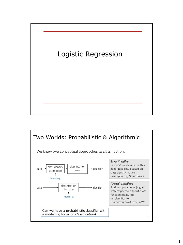
Logistic Regression Two Worlds: Probabilistic & Algorithmic We know two conceptual approaches to classification: Bayes es Classi ssifier er Probabilistic classifier with a classification class density data decision generative setup
Logistic Regression Two Worlds: Probabilistic & Algorithmic We know two conceptual approaches to classification: Bayes es Classi ssifier er Probabilistic classifier with a classification class density data decision generative setup based on rule estimation class density models Bayes (Gauss), Naïve Bayes learning “Direct” Classifiers classification Find best parameter (e.g. 𝑥 ) data decision function with respect to a specific loss function measuring learning misclassification Perceptron, SVM, Tree, ANN Can we have a probabilistic classifier with a modelling focus on classification ? 4 1
Advantages of Both Worlds • Posterior distribution has advantages over classification label: • Asymmetric risks: need classification probability • Classification certainty: Indicator if decision in unsure • Algorithmic approach with direct learning has advantages: • Focus of modelling power on correct classification where it counts • Easier decision line interpretation • Combination? 5 Discriminative Probabilistic Classifier Linear Classifier Bayes Classifier Discriminative Probabilistic Classifier Bishop PRML 𝑄 𝑦 𝐷 1 𝑄 𝑦 𝐷 2 Bishop PRML 𝑦 = 𝒙 𝑈 𝒚 + 𝑥 0 Ԧ 𝑄 𝐷 2 𝑦 ∝ 𝑄 𝑦 𝐷 2 𝑄 𝐷 2 6 2
Towards a “Direct” Probabilistic Classifier • Idea 1: Directly learn a posterior distribution For classification with the Bayes classifier, the posterior distribution is relevant. We can directly estimate a model of this distribution (we called this as a discriminative classifier in Naïve Bayes). We know from Naïve Bayes that we can probably expect a good performance from the posterior model. • Idea 2: Extend linear classification with probabilistic interpretation The linear classifier outputs a distance to the decision plane. We can use this value and interpret it probabilistically: “The further away, the more certain” 7 Logistic Regression The Logistic Regression will implement both ideas: It is a model of a posterior class distribution for classification and can be interpreted as a probabilistic linear classifier. But it is a fully probabilistic model, not only a “post - processing” of a linear classifier. It extends the hyperplane decision idea to Bayes world • Direct model of the posterior for classification • Probabilistic model (classification according to a probability distribution) • Discriminative model (models posterior rather than likelihood and prior) • Linear model for classification • Simple and accessible (we can understand that) • We can study the relation to other linear classifiers, i.e. SVM 8 3
History of Logistic Regression • Logistic Regression is a very “old” method of statistical analysis and in widespread use, especially in the traditional statistical community (not machine learning). 1957/58, Walker, Duncan, Cox • A method more often used to study and identify explaining factors rather than to do individual prediction. Statistical analysis vs. prediction focus of modern machine learning Many medical studies of risk factors etc. are based on logistic regression 9 10 Statistical Data Models We do not know P ( x,y ) but we can assume a certain form. ---> This is called a data model. Simplest form besides constant (one prototype) is a linear model . d T Lin x w x w w x , w w x w w i i 0 0 0 i 1 1 , w 0 x w x w Lin x w x , w w x , w 0 ► Linear Methods: Classification: Logistic Regression (no typo!) Regression: Linear Regression 4
Repetition: Linear Classifier Linear classification rule: 𝒚 = 𝒙 𝑈 𝒚 + 𝑥 0 𝒚 ≥ 0 ⇒ 𝒚 < 0 ⇒ Decision boundary is a a hyperplane 11 Repetition: Posterior Distribution • Classification with Posterior distribution: Bayes Based on class densities and a prior 𝑞 𝒚 𝐷 1 𝑄 𝐷 1 𝑞 𝒚 𝐷 2 𝑄 𝐷 2 𝑄 𝐷 1 𝒚 = 𝑄 𝐷 2 𝒚 = 𝑞 𝒚 𝐷 1 𝑄 𝐷 1 + 𝑞 𝒚 𝐷 2 𝑄 𝐷 2 𝑞 𝒚 𝐷 1 𝑄 𝐷 1 + 𝑞 𝒚 𝐷 2 𝑄 𝐷 2 Bishop PRML 12 5
Combination: Discriminative Classifier Decision boundary Bishop PRML Probabilistic interpretation of classification output: ~distance to separation plane 13 Notation Changes • We work with two classes Data with (numerical) feature vectors Ԧ 𝑦 and labels 𝒛 ∈ {𝟏, 𝟐} We do not use the notation of Bayes with 𝜕 anymore. We will need the explicit label value of 𝒛 in our models later. • Classification goal: infer the best class label {𝟏 𝒑𝒔 𝟐} for a given feature point 𝑧 ∗ = arg max 𝑧∈{0,1} 𝑄(𝑧|𝒚) • All our modeling focuses only on the posterior of having class 1 : 𝑄 𝑧 = 1 𝒚 • Obtaining the other is trivial: 𝑄 𝑧 = 0 𝒚 = 1 − 𝑄(𝑧 = 1 |𝒚 ) 14 6
Parametric Posterior Model We need a model for the posterior distribution, depending on the feature vector (of course) and neatly parameterized. 𝑄 𝑧 = 1 𝒚, 𝜾 = 𝑔 𝒚; 𝜾 The linear classifier is a good starting point. We know its parametrization very well: 𝒚; 𝒙, 𝑥 0 = 𝒙 𝑈 𝒚 + 𝑥 0 We thus model the posterior as a function of the linear classifier: 𝑄 𝑧 = 1 𝒚, 𝒙, 𝑥 0 = 𝑔(𝒙 𝑈 𝒚 + 𝑥 0 ) Posterior from classification result : “scaled distance“ to decision plane 15 Logistic Function To use the unbounded distance to the decision plane in a probabilistic setup, we need to map it into the interval [0, 1] This is very similar as we did in neural nets: activation function The logistic function 𝜏 𝑦 squashes a value 𝑦 ∈ ℝ to 0, 1 1 𝜏 𝑦 = 1 + e −𝑦 The logistic function is a smooth, soft threshold 𝜏 𝑦 → 1 𝑦 → ∞ 𝜏 𝑦 → 0 𝑦 → −∞ 𝜏 0 = 1 2 16 7
17 The Logistic Function 18 The Logistic “Regression” 8
The Logistic Regression Posterior We model the posterior distribution for classification in a two- classes-setting by applying the logistic function to the linear classifier: 𝑄 𝑧 = 1 𝑦 = 𝜏 𝑦 1 𝑄 𝑧 = 1 𝒚, 𝒙, 𝑥 0 = 𝑔(𝒙 𝑈 𝒚 + 𝑥 0 ) = 1 + 𝑓 −(𝒙 𝑈 𝒚+𝑥 0 ) This a location-dependent model of the posterior distribution, parametrized by a linear hyperplane classifier. 19 Logistic Regression is a Linear Classifier The logistic regression posterior leads to a linear classifier: 1 𝑄 𝑧 = 1 𝒚, 𝒙, 𝑥 0 = 1 + exp −(𝒙 𝑈 𝒚 + 𝑥 0 ) 𝑄 𝑧 = 0 𝒚, 𝒙, 𝑥 0 = 1 − 𝑄 𝑧 = 1 𝒚, 𝒙, 𝑥 0 𝑄 𝑧 = 1 𝒚, 𝒙, 𝑥 0 > 1 ⇒ 𝑧 = 1 classification; 𝑧 = 0 otherwise 2 𝑄 𝑧 = 1 𝒚, 𝒙, 𝑥 0 = 1 Classification boundary is at: 2 1 + exp −(𝒙 𝑈 𝒚 + 𝑥 0 ) = 1 1 𝒙 𝑈 𝒚 + 𝑥 0 = 0 ⇒ ⇒ 2 Classification boundary is a hyperplane 20 9
Interpretation: Logit Is the choice of the logistic function justified? • Yes, the logit is a linear function of our data: 𝑞 Logit: log of the odds ratio: ln 1−𝑞 ln 𝑄(𝑧 = 1|𝒚) The linear function (~distance from 𝑄(𝑧 = 0|𝒚) = 𝒙 𝑈 𝒚 + 𝑥 0 decision plane) directly expresses our classification certainty, measured by the “odds ratio”: double distance ↔ squared odds e.g. 3: 2 → 9: 4 • But other choices are valid, too They lead to other models than logistic regression, e.g. probit regression 𝐹[𝑧] = 𝑔 −1 𝒙 𝑈 𝒚 + 𝑥 0 → Generalized Linear Models (GLM) 21 22 The Logistic Regression • So far we have made no assumption on the data! • We can get r ( x ) from a generative model or model it directly as function of the data (discriminative) Logistic Regression: 𝑄(𝑧=0|𝒚) = log 𝑄(𝑧=1|𝒚) 𝑞 Model: The logit r ( x ) = log 1−𝑞 is a linear function of the data d p r x log w x w w x , i i 0 1 p i 1 1 P y P y 1 1 x x w x w x , , < = > 1 exp w x , 10
Training a Posterior Distribution Model The posterior model for classification requires training. Logistic regression is not just a post-processing of a linear classifier. Learning of good parameter values needs be done with respect to the probabilistic meaning of the posterior distribution. • In the probabilistic setting, learning is usually estimation We now have a slightly different situation than with Bayes: We do not need class densities but a good posterior distribution . • We will use Maximum Likelihood and Maximum-A-Posteriori estimates of our parameters 𝒙, 𝑥 0 Later: This also corresponds to a cost function of obtaining 𝒙, 𝑥 0 23 Maximum Likelihood Learning The Maximum Likelihood principle can be adapted to fit the posterior distribution (discriminative case): • We choose the parameters 𝒙, 𝑥 0 which maximize the posterior distribution of the training set 𝒀 with labels 𝒁 : 𝒙, 𝑥 0 = arg max 𝒙,𝑥 0 𝑄 Y 𝑌; 𝒙, 𝑥 0 ς 𝒚∈𝑌 𝑄 𝑧 𝒚; 𝒙, 𝑥 0 = arg max (iid) 𝒙,𝑥 0 𝒚; 𝒙, 𝑥 0 𝑧 𝑄 𝑧 = 0 𝒚; 𝒙, 𝑥 0 1−𝑧 𝑄 𝑧 𝒚; 𝒙, 𝑥 0 = 𝑄 𝑧 = 1 24 11
Recommend
More recommend
Explore More Topics
Stay informed with curated content and fresh updates.
