Linear discriminant functions Andrea Passerini - PowerPoint PPT Presentation
Linear discriminant functions Andrea Passerini passerini@disi.unitn.it Machine Learning Linear discriminant functions Discriminative learning Discriminative vs generative Generative learning assumes knowledge of the distribution governing
Linear discriminant functions Andrea Passerini passerini@disi.unitn.it Machine Learning Linear discriminant functions
Discriminative learning Discriminative vs generative Generative learning assumes knowledge of the distribution governing the data Discriminative learning focuses on directly modeling the discriminant function E.g. for classification, directly modeling decision boundaries (rather than inferring them from the modelled data distributions) Linear discriminant functions
Discriminative learning PROS When data are complex, modeling their distribution can be very difficult If data discrimination is the goal, data distribution modeling is not needed Focuses parameters (and thus use of available training examples) on the desired goal CONS The learned model is less flexible in its usage It does not allow to perform arbitrary inference tasks E.g. it is not possible to efficiently generate new data from a certain class Linear discriminant functions
Linear discriminant functions Description f ( x ) = w T x + w 0 The discriminant function is a linear combination of example features w 0 is called bias or threshold it is the simplest possible discriminant function Depending on the complexity of the task and amount of data, it can be the best option available (at least it is the first to try) Linear discriminant functions
Linear binary classifier Description f ( x ) = sign ( w T x + w 0 ) It is obtained taking the sign of the linear function The decision boundary ( f ( x ) = 0) is a hyperplane ( H ) The weight vector w is orthogonal to the decision hyperplane: ∀ x , x ′ : f ( x ) = f ( x ′ ) = 0 w T x + w 0 − w T x ′ − w 0 = 0 w T ( x − x ′ ) = 0 Linear discriminant functions
Linear binary classifier Functional margin The value f ( x ) of the function for a certain point x is called functional margin It can be seen as a confidence in the prediction Geometric margin The distance from x to the hyperplane is called geometric margin r x = f ( x ) || w || It is a normalize version of the functional margin The distance from the origin to the hyperplane is: r 0 = f ( 0 ) || w || = w 0 || w || Linear discriminant functions
Linear binary classifier Geometric margin (cont) A point can be expressed by its projection on H plus its distance to H times the unit vector in that direction: x = x p + r x w || w || Linear discriminant functions
Linear binary classifier Geometric margin (cont) Then as f ( x p ) = 0: w T x + w 0 f ( x ) = w T ( x p + r x w = || w || ) + w 0 w w T x p + w 0 + r x w T = || w || � �� � f ( x p ) r x || w || = f ( x ) r x = || w || Linear discriminant functions
Biological motivation Human Brain Composed of densely interconnected network of neurons A neuron is made of: soma A central body containing the nucleus dendrites A set of filaments departing from the body axon a longer filament (up to 100 times body diameter) synapses connections between dendrites and axons from other neurons Linear discriminant functions
Biological motivation Human Brain Electrochemical reactions allow signals to propagate along neurons via axons, synapses and dendrites Synapses can either excite on inhibit a neuron potentional Once a neuron potential exceeds a certain threshold , a signal is generated and transmitted along the axon Linear discriminant functions
Perceptron Single neuron architecture f ( x ) = sign ( w T x + w 0 ) Linear combination of input features Threshold activation function Linear discriminant functions
Perceptron Representational power Linearly separable sets of examples E.g. primitive boolean functions (AND,OR,NAND,NOT) ⇒ any logic formula can be represented by a network of two levels of perceptrons (in disjunctive or conjunctive normal form). Problem non-linearly separable sets of examples cannot be separated Representing complex logic formulas can require a number of perceptrons exponential in the size of the input Linear discriminant functions
Perceptron Augmented feature/weight vectors w T ˆ f ( x ) = sign ( ˆ x ) Where bias is incorporated in augmented vectors: � w 0 � 1 � � ˆ ˆ w = x = w x Search for weight vector + bias is replaced by search for augmented weight vector (we skip the “ ˆ ” in the following) Linear discriminant functions
Parameter learning Error minimization Need to find a function of the parameters to be optimized (like in maximum likelihood for probability distributions) Reasonable function is measure of error on training set D (i.e. the loss ℓ ): � E ( w ; D ) = ℓ ( y , f ( x )) ( x , y ) ∈D Problem of overfitting training data (less severe for linear classifier, we will discuss it) Linear discriminant functions
Parameter learning Gradient descent Initialize w (e.g. w = 0) 1 Iterate until gradient is approx. zero: 2 w = w − η ∇ E ( w ; D ) Note η is called learning rate and controls the amount of movement at each gradient step The algorithm is guaranteed to converge to a local optimum of E ( w ; D ) (for small enough η ) Too low η implies slow convergence Techniques exist to adaptively modify η Linear discriminant functions
Parameter learning Problem The misclassification loss is piecewise constant Poor candidate for gradient descent Perceptron training rule � E ( w ; D ) = − yf ( x ) ( x , y ) ∈D E D E is the set of current training errors for which: yf ( x ) ≤ 0 The error is the sum of the functional margins of incorrectly classified examples Linear discriminant functions
Parameter learning Perceptron training rule The error gradient is: � ∇ E ( w ; D ) = ∇ − yf ( x ) ( x , y ) ∈D E � − y ( w T x ) = ∇ ( x , y ) ∈D E � = − y x ( x , y ) ∈D E the amount of update is: � − η ∇ E ( w ; D ) = η y x ( x , y ) ∈D E Linear discriminant functions
Perceptron learning Stochastic perceptron training rule Initialize weights randomly 1 Iterate until all examples correctly classified: 2 For each incorrectly classified training example ( x , y ) 1 update weight vector: w ← w + η y x Note on stochastic we make a gradient step for each training error (rather than on the sum of them in batch learning) Each gradient step is very fast Stochasticity can sometimes help to avoid local minima, being guided by various gradients for each training example (which won’t have the same local minima in general) Linear discriminant functions
Perceptron learning Linear discriminant functions
Perceptron learning Linear discriminant functions
Perceptron learning Linear discriminant functions
Perceptron learning Linear discriminant functions
Perceptron learning Linear discriminant functions
Perceptron regression Exact solution R n × I R d be the input training matrix (i.e. Let X ∈ I X = [ x 1 · · · x n ] T for n = |D| and d = | x | ) R n be the output training matrix (i.e. y i is output for Let y ∈ I example x i ) Regression learning could be stated as a set of linear equations): X w = y Giving as solution: w = X − 1 y Linear discriminant functions
Perceptron regression Problem Matrix X is rectangular, usually more rows than columns System of equations is overdetermined (more equations than unknowns) No exact solution typically exists Linear discriminant functions
Perceptron regression Mean squared error (MSE) Resort to loss minimization Standard loss for regression is the mean squared error: � ( y − f ( x )) 2 = ( y − X w ) T ( y − X w ) E ( w ; D ) = ( x , y ) ∈D Closed form solution exists Can always be solved by gradient descent (can be faster) Can also be used as a classification loss Linear discriminant functions
Perceptron regression Closed form solution ∇ ( y − X w ) T ( y − X w ) ∇ E ( w ; D ) = 2 ( y − X w ) T ( − X ) = 0 = − 2 y T X + 2 w T X T X = 0 = w T X T X y T X = X T X w X T y = ( X T X ) − 1 X T y = w Linear discriminant functions
Perceptron regression w = ( X T X ) − 1 X T y Note ( X T X ) − 1 X T is called left-inverse If X is square and nonsingular, inverse and left-inverse coincide and the MSE solution corresponds to the exact one R d × d is full rank The left-inverse exists provided ( X T X ) ∈ I → features are linearly independent (if not, just remove the redundant ones!) Linear discriminant functions
Perceptron regression Gradient descent ∂ E ∂ 1 � ( y − f ( x )) 2 = ∂ w i ∂ w i 2 ( x , y ) ∈D = 1 ∂ � ( y − f ( x )) 2 2 ∂ w i ( x , y ) ∈D = 1 2 ( y − f ( x )) ∂ � ( y − w T x ) 2 ∂ w i ( x , y ) ∈D � = ( y − f ( x ))( − x i ) ( x , y ) ∈D Linear discriminant functions
Multiclass classification One-vs-all Learn one binary classifier for each class: positive examples are examples of the class negative examples are examples of all other classes Predict a new example in the class with maximum functional margin Decision boundaries for which f i ( x ) = f j ( x ) are pieces of hyperplanes: w T w T = i x j x ( w i − w j ) T x = 0 Linear discriminant functions
Multiclass classification Linear discriminant functions
Multiclass classification all-pairs Learn one binary classifier for each pair of classes: positive examples from one class negative examples from the other Predict a new example in the class winning the largest number of pairwise classifications Linear discriminant functions
Recommend
More recommend
Explore More Topics
Stay informed with curated content and fresh updates.
